CalDB 4.4.1 Public Release Notes
SDP Release Date: 22 DEC 2010
Public Release: 15 DEC 2010
I. INTRODUCTION:
CalDB 4.4.1 is a significant upgrade to CalDB 4.3.1 and later versions, which includes the following items:
- ACIS Contamination File Version 6 with upgrade for ACIS-I modeling.
- ACIS Subpixel Repositioning File (SUBPIX) CalDB File.
- ACIS T_GAIN Epoch 43 (Aug-Oct 2010).
- ACIS-S/LETG LSFPARMs Version 4
- HRC-I GMAP for 2010-09-25
- HRC-I QE Version 8 update for consistency with HRC-S and LETG/ACIS-S.
- HRC-S SAMP-based RMF Version 1 for quantiles, hardness ratios, and background reduction.
CalDB 4.4.1 includes two sets of upgrades, one for CalDB 4.4.0, and the other properly for 4.4.1, released with CIAO 4.3.
For the CIAO 4.3 release notes, and How CalDB 4.4.1 Affects Your Analysis, see this link.
II. SUMMARY OF CHANGES
A. ACIS Contamination File Version 6
| Location: | $CALDB/data/chandra/acis/contam/ |
| Filename: | acisD1999-08-13contamN0006.fits |
The ACIS-I contamination model has been upgraded to a similar model to the ACIS-S upgrade in version N0005, released in December 2009. The new model uses a different handling of the amorphous component, while retaining the edge structures included in the original contaminant model. Both the ACIS-I and ACIS-S portions have been extended in time, so that the interpolations are valid now through mid-2014.
See the ACIS QE Contamination Why? Page for more information. Technical details concerning the new CalDB data file are given in the section below.
PIPELINES/TOOLS AFFECTED:
CIAO 4.3 (with ACIS-related data only): mkarf, mkwarf, fullgarf, mkinstmap
THREADS AFFECTED:
Extract Spectrum and Response Files for a Pointlike Source
Extract Spectrum and Response Files
for an Extended Source
Extract Spectrum and Response Files
for Multiple Sources
HETG/ACIS-S Grating
ARFs
LETG/ACIS-S Grating
ARFs
Object-centered Aspect
Solution and Exposure Map
B. ACIS Subpixel Repositioning File
| Location: | $CALDB/data/chandra/acis/subpix/ |
| Filename: | acisD1999-07-22subpixN0001.fits |
The ACIS energy-dependent subpixel event repositioning algorithm requires subpixel shift data as a function of photon energy associated with three different event types, to which each of the good flight grades (FLTGRADE) may be assigned. Once done, the respective event positions may be shifted by the prescribed amount. The shift data have been derived and published in the recent literature, and smoothed to derive the data used in the CalDB file.
The ACIS EDSER algorithm will not be implemented in Standard Data Processing until version DS 8.4 is released.
See the ACIS Subpixel Event Repositioning Why? page, and the technical details section below for more information.
PIPELINES/TOOLS AFFECTED:
ACIS Level 1 Pipeline tool acis_process_events
ACIS full reprocessing script chandra_repro
THREADS AFFECTED:
See the analysis guide: ACIS Sub-Pixel
Event Resolution Analysis Guide for lists of applicable Chart threads, including:
Creating an Image of the PSF
C. ACIS T_GAIN Epoch 43
| Location: | $CALDB/data/chandra/acis/t_gain/ |
| Filenames: | acisD2010-05-01t_gainN0006.fits acisD2010-05-01t_gainN0005.fits acisD2010-08-01t_gain_biN0002.fits acisD2010-08-01t_gainN0002.fits |
With the completion of the ACIS ECS radiation-zone CTI-monitoring observations for T_GAIN Epoch 43 (August through October 2010), the ACIS calibration team has filtered and prepared the latest corrections for the time-varying gain versus energy. These are then applied in SDP and CIAO reprocessing with acis_process_events by interpolation between successive epochs. Hence there are always four new files introduced with each T_GAIN upgrade. The technical details are given below.
See the ACIS Time-dependent Gain Why page for more information.
PIPELINES/TOOLS AFFECTED:
THREADS AFFECTED:
Reprocessing Data to create a New L2 Events File
D. ACIS-S/LETG LSFPARMs Version 4
| Location: | $CALDB/data/chandra/acis/lsfparm/ |
| Filenames: | acissleg-1D1999-07-22lsfparmN0004.fits acissleg1D1999-07-22lsfparmN0004.fits |
Now that there has been a correction installed for the long-standing LETG/ACIS-S grating tilt angle, it is possible to implement a more precise and limiting LSF parameter file for that configuration. See the technical details for these new LSFPARM files below.
PIPELINES/TOOLS AFFECTED:
mkgrmf for the LETG/ACIS-S configuration only.
THREADS AFFECTED:
E. HRC-I GMAP for 2010-09-25
| Location: | $CALDB/data/chandra/hrc/gmap/ |
| Filenames: | hrciD2010-09-25sampgainN0001.fits |
With the release of CalDB 4.2.0 in December 2009, a new metric for HRC-I gain correction was introduced, called the SUMAMPS-based gain map (SAMP GMAP). The SUMAMPS metric (the sum of the three nearest amplifier signals) is better than PHA (sum of all amp signals) because it gives less small-scale spatial variation, and allows for a better gain correction. The new file is to be added because of the continued time-dependent variation in the HRC-I gain, which programmatically is optimized approximately annually. For details on the derivation of the new GMAP see the tech details section below.
PIPELINES/TOOLS AFFECTED:
SDP/CIAO HRC Level 1 event (re)processing tool hrc_process_events.
THREADS AFFECTED:
Creating new HRC-I L2 events file
F. HRC-I QE Version 8
| Location: | $CALDB/data/chandra/hrc/qe/ |
| Filenames: | hrciD1999-07-22qeN0008.fits |
The HRC-I QE versus energy has been upgraded to make it consistent with changes in the HRC-S and ACIS-S quantum efficiency curves released in December 2009. See the technical details below for a figure to demonstrate the degree of the changes as a function of energy versus the previous QE.
PIPELINES/TOOLS AFFECTED:
CIAO tool mkinstmap (mkexpmap) for the HRC-I.
THREADS AFFECTED:
HRC-I Exposure Map and Fluxed Image
G. HRC-S SAMP-based RMF Version 1
| Location: | $CALDB/data/chandra/hrc/rmf/ |
| Filenames: | hrcsD1999-07-22samprmfN0001.fits |
A new SAMP-based RMF for HRC-S has now been released, suitable for calculating quantiles, hardness ratios, and for use in background reduction, for observations that have been processed with the time-dependent GMAP (T_GMAP) released in December 2009. See details regarding the RMF and its uses in the technical details section below. WARNING: This RMF is not to be used for spectral fitting of HRC-S data; the energy resolution in HRC-S is too poor to allow a reasonably-defined energy scale. If you do elect to use this RMF for spectral fitting, you are strongly advised to work in PHA space, and not PI space.
The new SAMP-based RMF is described in the Technical Details section below.
THREADS AFFECTED:
Currently there are no CIAO threads for the use of the HRC-S RMF. However, please see the HRC-S RMF calibration page for more details on quantile color-color mapping with this RMF.
III. TECHNICAL DETAILS
A. ACIS Contamination File Version 6
We have added an upgrade of the ACIS-I Optical Blocking Filter (OBF) contamination model to the ACIS CONTAM file in CalDB. We have also extended the validity of the ACIS-S model until Mid-2014. The new ACIS-I model is very similar to the ACIS-S model included in the N0005 CONTAM file released in December of 2009 (last year). The new model is mainly derived to give consistent model fits to galaxy cluster spectra taken over the full Chandra mission timeline, most specifically from Abell 1795.
In particular, the new model, which wasn't working well with cluster data taken with variations in the focal plane temperature of ACIS from one OBS_ID to another, has been found to work much better in fitting the data once the temperature-dependent CTI correction is applied. That new T-CTI correction is now available in CIAO 4.3, and is being applied in Standard Data Processing since 02 November 2010.
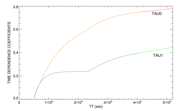
The ACIS-S contamination model in the version N0005 file was released with a somewhat limited interpolation range in time in Dec 2009. For the new N0006 release in Dec 2010, the interpolation range has been extended to mid-2014. This was done by extrapolating the time-dependent coefficients as in Fig. 1 below.
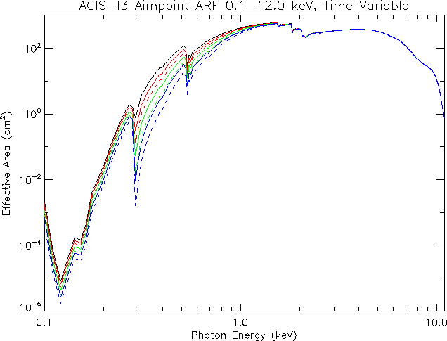
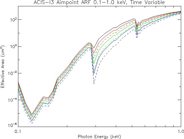
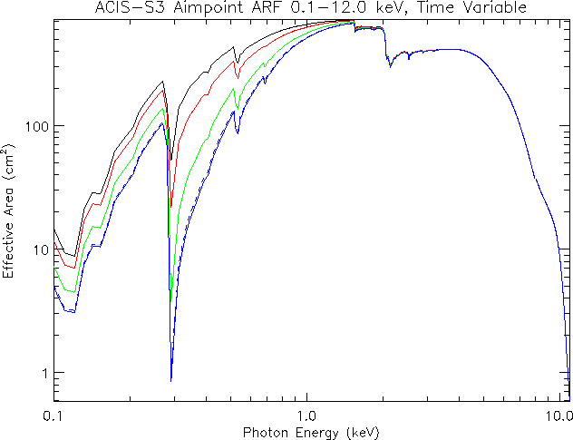
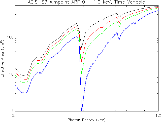
Illustrations of the ACIS-I and ACIS-S aim-point effective areas with the new versus the previous CONTAM files are shown in Figs 3 and 4 below. Note that the ACIS-S results show no variation between N0005 and N0006 until the 15 May 2014 traces, where the difference is due to the extrapolation of the time base in the N0005 file. For ACIS-I, the newer model gives a somewhat different shape versus energy, as well as a little less absorption in the C-K range, than the old one.
|
|
|
|
|
|
Finally, see the four plots in coma-comparison.pdf, which illustrate the efficacy of the new ACIS-I CONTAM model for the Coma Cluster with and without the ACIS temperature-dependent CTI correction. The new model correctly fits the temperature-corrected data, but not the data without the T-CTI correction. This is the most essential justification we have found for releasing the new CONTAM model upgrade for ACIS-I.
B. ACIS Subpixel Repositioning File
The ACIS Energy Dependent Subpixel Event Repositioning (EDSER) algorithm has been implemented in acis_process_events for CIAO 4.3, released 15 December 2010. The software requires analysis reference data, the new ACIS SUBPIX file in CalDB 4.4.1
The specification for the EDSER algorithm and a brief description of the ARD are given in the CXC SDS memorandum http://space.mit.edu/ASC/docs/subpix_spec_1.2.pdf.
The basic contents of the file have been derived and published in the literature for both the ACIS FI and BI chips. (See Jingqiang Li, Joel H. Kastner, Gregory Y. Prigozhin, and Norbert S. Schulz, ApJ 590:586-592, 2003 June 10, as well as Li, et al, ApJ 610:1204-1212, 2004 August 1.)
Specifically, the file acisD1999-07-22subpixN0001.fits, includes 10 BINTABLE blocks, one for each ACIS chip. For the 8 FI chips each block has the same BINTABLE dataset, and similarly for the two BI chips. The data for the BI and FI chips comes from Li, et al, ApJ 610:1204-1212, 2004 August 1, Figure 4, included below as Fig. 6 for illustration.
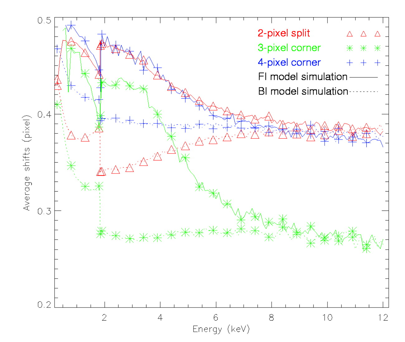
Because of noise in the traces in the plot, G. Allen has smoothed the data in the traces to reduce it to an applicable table format. Each of the 256 flight grade event types has been assigned to one of the three curves, so that those shift values might be applied appropriately in the a-p-e EDSER algorithm.
At this time, no such data have been implemented for the CC mode data, and hence the file and algorithm will not be applied to CC mode data in this release.
NOTE regarding Standard Data Processing: The EDSER algorithm will not be implemented in SDP for some months; however the new CalDB with this subpix file can be installed in SDP without affecting operations until the subpix EDSER software is implemented in the DS acis_process_events. The file will be present in CalDB, but not used in SDP until a later DS installation is done.
C. ACIS T_GAIN Epoch 43
The ACIS time-dependent gain corrections (T_GAIN) have recently been updated for current changes from the previous T_GAIN epoch, specifically Epoch 43, which was August through October 2010. With the addition of these new corrections, derived from ACIS External Cal Source (ECS) data taken during radiation zone passes, the CalDB files extending from May through July 2010 (i.e. Epoch 42) have been finalized, and new non-interpolating T_GAIN files are now implemented for Epoch 43.
The magnitudes (in eV) of the new gain corrections, versus photon energy, are given in Figs. 6-8 below. The corrections are of the usual order in magnitude, specifically less than 0.5% of the photon energy value. Fig. 6 below gives the corrections for the ACIS-I aimpoint on chip ACIS-3, for the CTI-corrected case, which is the only one applicable to FI chips. Figure 7 gives the corrections for the ACIS-S aimpoint on ACIS-7, for the case where the BI chips are NOT CTI-corrected (e.g. for GRADED datamodes). Finally Fig. 8 gives the corrections for ACIS-7 for CTI-corrected BI chips.

D. ACIS-S/LETG LSFPARMs Version 4
The long-standing ACIS-S/LETG grating tilt error (0.086 degrees) was fixed with installation of new PIXLIB files in CalDB 4.4.0. This enables use of a narrower spectral extraction region (the SDP default is now |tg_d|<0.0008 rather than 0.0020), with reduced background contamination. At the same time, the LETG calibration team has released new grating extraction efficiencies (EEFRACS) as part of two new LSFPARM (LSF parameter) files for +1 and -1 orders. From the Calibration Group (Brad Wargelin):
- New LSFPARMS files for the LETG/ACIS, containing improved EEFRACS
(spectral extraction efficiencies). The files are
acissleg-1D1999-07-22lsfparmN9999saosac+obs.fits
(renamed to acissleg-1D1999-07-22lsfparmN0004.fits for CalDB)
acissleg1D1999-07-22lsfparmN9999saosac+obs.fits
(renamed to acissleg1D1999-07-22lsfparmN0004.fits for CalDB).
- The new EEFRACS differ from the old in that:
- They were obtained from SAOSAC simulations instead of vanilla MARX. The main effect was to increase scattering in the wings a little.
- The old EEFRACS were improperly normalized to counts falling on the detector, rather than to all counts over 2*pi. This is only a significant effect at rather long wavelengths, beyond the useful wavelength range for LETG/ACIS.
- The new SAOSAC results were then empirically adjusted to better match observations, which show a significantly broader core and higher flux in the scattering wings. The net result is to lower EEFRACS by ~3% for the (new, narrower, |tg_d|<0.0008) spectral extraction region relative to the old EEFRACS. There is less than a 1% difference when using the old (wider, |tg_d|<0.0020) spectral extraction region, however.
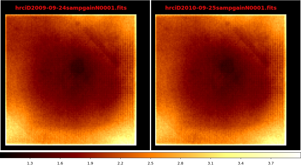
E. HRC-I GMAP for 2010-09-25
A new update for the time-varying gain map (GMAP) of the HRC-I has been released by the HRC-I calibration team, effective 2009-09-25T12:00:00. The new file is called hrciD2010-09-25sampgainN0001.fits. It is a SUMAMPS-based gain map, which is the standard for HRC. For both the HRC-I and HRC-S, the scaled sum of amplifier signals (SUMAMPS) is a better proxy for spectral response than the PHA.
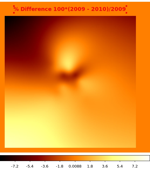
An illustration of the new GMAP is given in Fig. 10 below, with a comparison for the previous one that has been effective since 2009-09-24. The units of the image are arbitrary, due to the scaling of the SUMAMPS values. A hidden scale factor of 148 (for HRC-I) is used to rescale the SUMAMPS values to make them roughly similar to the PHA. The GMAP is then applied to get PIs, which are set to appear in the 1-1024 range. A difference plot between the two GMAPs is given in Fig. 11. The new map varies by as much as -9/% (upper left corner of the map), but in other regions gives +6/% differences (the lightest-colored regions). These are typical annual variations for the HRC-I GMAPs.
In Fig. 12 below, is an illustration of the difference in the calculated PI values (all events included) for a particular OBS_ID of AR Lac. Note that the range of PI's increases with the new GMAP, indicating the gain reduction with time for this source near the aimpoint of HRC-I.
The file was constructed by the HRC-I Cal Team and delivered on 2010-11-01 for inclusion in the next CalDB release. The procedure is outlined in the memorandum "SUMAMPS-based Gain Maps for the HRC-I" and posted online at
http://cxc.harvard.edu/cal/Hrc/Documents/Gain/hrci_sampgain_nov2009.pdf
F. HRC-I QE Version 8
The HRC-I N0008 QE upgrade is described in the Calibration Web page An Update to the HRC-I MCP QE Model. From that posting:
| The normalization of the in-flight HRC-I microchannel plate (MCP) quantum efficiency (QE) model is determined by cross-calibration with the HRC-S/LETG and ACIS using common calibration sources. In the past two years, the HRMA effective area model, ACIS contamination model, and HRC-S QE model have been updated, prompting us to update the HRC-I QE model. This page documents the creation of this newest QE model, version N0008. |
The HRC-I QE has been upgraded by the following procedure, as described in detail and illustrated in the above web page:
- Updated the low-energy MCP QE(E) below 626 eV using the HRC-S QE
as shaping factor.
- The UVIS-I curve must be divided out of the HRC-I QE N0007 curve to obtain the raw MCP QE(E).
- The HRC-S MCP QE at 626 eV and below, with a shifting factor in QE, is "pasted" onto the HRC-I QE curve above 626 eV.
- Checked the modified HRC-I QE model normalization using standard cosmic calibration sources G21.5-0.9, PKS 2155-304, and HZ 43. The analysis was done in CIAO 4.2. G21.5-0.9 measurements and predicted fluxes were derived using ACIS-S3 observations, with the ACIS CONTAM model version N0005 released in CalDB 4.2.0.
- Renormalized the HRC-I QE model for appropriate fluxes from the
standard sources.
- Beginning with the pasted low-energy section of the curve, repeat the normalization using HRC-S/LETG and HRC-I/LETG measurements of sources HZ 43 and PKS 2155-304.
- Use a broadened step function to renormalize the remainder of the QE(E) (i.e. for E > 626 eV). The parameters of the function are chosen to minimize the difference between measured and predicted count rates for all three of the standard sources, using the repasted HRC-I QE.
The resulting new HRC-I QE(E) is given in Fig. 13 below, with UVIS-I reapplied. A difference plot between the N0007 (old) and N0008 (new) QE(E) is given Fig. 14. In both figures, the trace referred to as "repaste" is the intermediate model from step 3a above, before the modified step function is applied to get the N0008 curve. Both plots were taken from the HRC-I QE upgrade web page above.

|
|
|
Fig. 13: HRC-I QE comparison of the N0007, renormalized-pasted, and N0008 traces. |
Fig. 14: Difference ratios of the renormalized-repasted and N0008 QE models versus N0007. |
G. HRC-S SAMP-based RMF Version 1
Now that the time-dependent gain map for HRC-S, based on the
SUMAMPS-derived PI rather than the PI based on PHA, there is a need
for an appropriate RMF upgrade. From the HRC-S Calibration Team, posted at web page:
http://cxc.harvard.edu/cal/Hrc/RMF/samp_rmf.html#s
"The spectral resolution of the HRC-S in imaging mode is poor
compared to that of the ACIS detectors, but the HRC-S does exhibit a
non-linear response to photon energies that can be advantageous in
characterizing spectral hardness. To facilitate this, we have
constructed a Redistribution Matrix file (RMF) that can be used in
either Sherpa or XSPEC. A previous version of the RMF was constructed
for use with 256-channel PI that was derived using PHA. The new
version is for use with SAMP-derived 1024-channel PI values. For more
information about the gain map used to convert SAMP to PI, see 'HRC-S
Gain Map and LETG Background Filter,' at
http://cxc.harvard.edu/cal/Letg/Hrc_bg/."
To generate the RMF, HRC-S/LETG observations of Capella, PKS 2155-304, RXJ1856.5-3754, V4743 Sgr, and Mkn 421 were used to measure the spectral response for various photon energies. The data were reprocessed with hrc_process_events (CIAO 4.2, CalDB 4.2) to apply the time-dependent HRC-S GMAP. The grating L1.5 and L2 processing was then run to assign a wavelength to each event based on position on the HRC-S array.
The data were then filtered on the respective energy ranges as specified in Table 1 of the HRC-S Web page above, and binned in wavelength to obtain at least 4000 counts per bin. The bin sizes ranged from 0.02 to 1.2 Angstroms. At this point, 2-D arrays for both source and background could be assembled in wavelength/PI space, with 1-channel PI bins. After Loess-smoothing in both dimensions, the smoothed background array (multiplied by extraction area ratio) was subtracted from the smoothed source array. The result was then normalized so that the sum over each wavelength bin was 1. Hence the resulting RMF:
