An Update to the HRC-I MCP QE Model
Jennifer Posson-Brown & Vinay Kashyap
October 2010
Abstract
We present an updated model (N0008) for the HRC-I MCP quantum efficiency.
This model, released in the December 2010 CALDB, is based on cross-calibration with the HRC-S and
ACIS and includes the effects of updated response models for those
instruments. The calibration sources used are HZ 43 (soft band), PKS
2155-304 (medium band) and G21.5-0.9 (hard band).
Contents:
- Introduction
- Updating the model shape at low energies
- Checking the model normalization
- Renormalizing the model
- Summary
- Appendix: Checking cross-calibration with E0102
(added July 2012)
1. Introduction
The normalization of the in-flight HRC-I microchannel plate (MCP)
quantum efficiency (QE) model is determined by
cross-calibration with the HRC-S/LETG and ACIS using common
calibration sources. In the past two years, the HRMA effective area
model, ACIS contamination model, and HRC-S QE model have been updated,
prompting us to update the HRC-I QE model. This page documents the
creation of this newest QE model, version N0008, which will be in the
December 2010 CALDB release.
2. Updating the model shape at low energies
In 2002, as part of a modification to the HRC-I QE, the HRC-S QE was
used as a "shaping factor" below 626 eV, where the response was not
well-known in the original flight model. This is documented in the memo "A New Flight Model of the
HRC-I MCP Quantum Efficiency" (Hole, K T, Donnelly, R H &
Posson-Brown, J, 2002). Since a revised HRC-S QE model was released
in December 2009 (CALDB 4.2.0), our first step in updating the HRC-I
QE model was to redo this "low-energy paste".
The figure below shows a comparison of the current HRC-S and old HRC-I
QE models -
hrciD1999-07-22qeN0007.fits (red dotted line) and
hrcsD1999-07-22qeN0010.fits (blue dashed line). Note that the HRC-S
QE plotted here is for chip 2, region 203 (where the HRC-S aimpoint is
located.) These models include the UVIS transmission
efficiency models UVIS-I v4 and UVIS-S1 (a.k.a "center thick section")
v4, respectively. The solid lines show the QE models (blue=S, pink=I)
with the UVIS efficiencies removed.
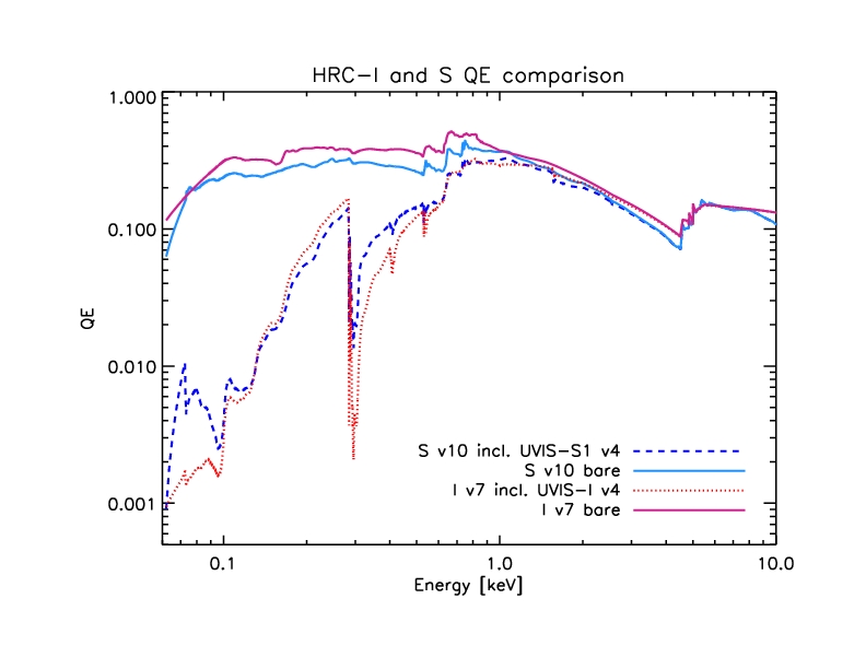
Figure 1: HRC-I and S QE models with and without UVIS efficiency.
The following figure compares the UVIS-I (red) and -S1 (blue)
models:

Figure 2: UVIS efficiency models
Note that the "low-energy paste" will be done with the bare MCP QE
models, not including UVIS efficiencies.
The following plot shows the HRC-I and S MCP QE models (pink and blue
lines), with the dashed green line showing the HRC-S model raised to
match the HRC-I model around 626 eV. (The red X shows the point where
we will do the paste.)
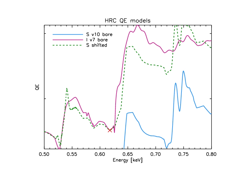
Figure 3: Close-up of "low-energy paste"
Model with new paste:
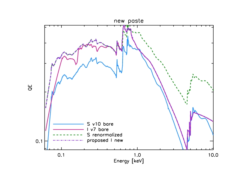
Figure 4: HRC-I MCP model with new low-energy paste (purple
dot-dash line).
After redoing this low-energy paste, the UVIS-I efficiency is folded
back in, and the resulting QE is saved as hrciD1999-07-22qeN0007prime.fits.
3. Checking QE model normalization
To check the normalization of the HRC-I QE model, we use HRC-S/LETG
and ACIS observations of common sources to generate source models. We
use these source models and HRC-I ARFs to predict HRC-I count rates.
We then compare the predicted rates to observed HRC-I count rates. We
have used three calibration sources for this effort: SNR G21.5-0.9,
blazar PKS 2155-304, and white dwarf HZ 43. Each of these sources are
discussed in detail below. A summary of the calibration observations used in this analysis is
shown in Table 1. A summary of observed count rates and predicted count rates with
models N0007 and N0007prime is shown in Table 2.
3.1 Hard Band: G21.5-0.9
3.1.1 Observed HRC-I Count Rates
The observed count rates are taken from reprocessed level=2 event
files, filtered using the ciao deflare tool to remove times
affected by high background rates. Source counts are extracted from a
circular region with radius 43" centered on the pulsar and background
counts are taken from a large annulus with inner radius 10' and outer
radius 12'.
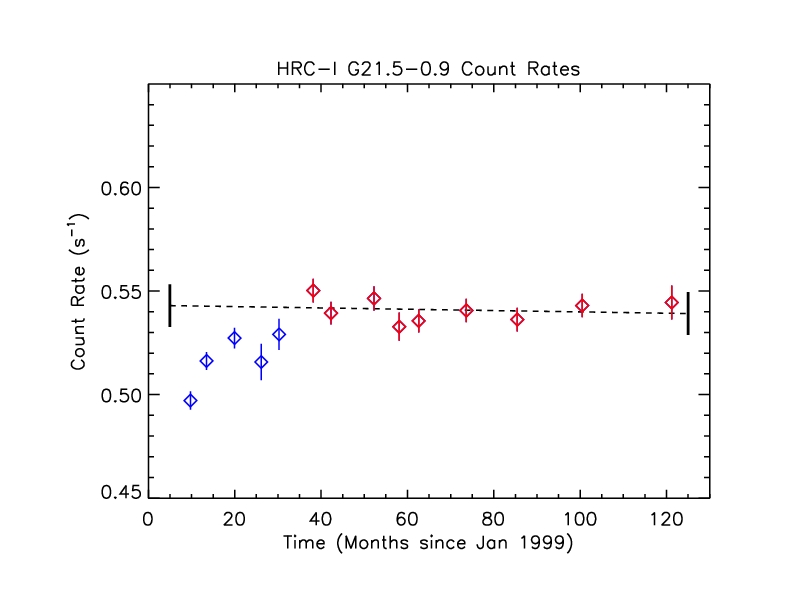
Figure 5: Observed G21.5-0.9 count rates
Count rates from the first several observations are depressed for
reasons we do not yet understand. For the purposes of
cross-calibration to renormalize the HRC-I QE model, we do a linear fit to the
points shown in red, beginning around t=40 months. The best-fit line
has a slope that is consistent with zero (-3.205e-05 +/- 8.270e-05
cts/s/month)
and y-intercept of 0.543 +/- 0.006 cts/s (errors are 1 sigma). The mean
rate is 0.541 cts/s with standard deviation 0.006. The mean of the errors
is 0.006.
3.1.2 Source Model
To generate a source model for G21.5-0.9, we used three ACIS-S3
subarray observations (ObsIDs 1553, 1554 and 3693). We choose to use
the subarray observations as they are not affected by pileup. The
data were reprocessed with CIAO 4.2. Source counts were extracted
from a circular region with radius 43" centered on the pulsar and
background counts were extracted from an identical sized region
located at least 165" away from the pulsar. The spectra and response
files were generated using specextract
We jointly fit the three spectra in XSPEC with an absorbed powerlaw
model (TBabs*pegpwrlw, abund=wilm, xsect=vern) over the 1-8 keV band.
The eMin and eMax parameters of the pegpwrlw model are frozen to 2.0
and 8.0 keV. The spectra, best-fit model and residuals are shown in the following
plot:
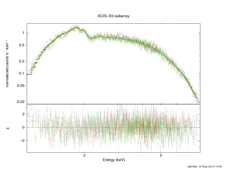
Figure 5: Fit to ACIS-S3 observations of G21.5-0.9.
We obtain best-fit parameters of nH = 3.23466 x 10^22 cm^-2
[3.20203, 3.26783], PhoIndex = 1.79686 [1.78078, 1.81308] and
norm = 54.9971 x 10^-12 erg cm^-2 s^-1 [54.7394, 55.2557] (90%
confidence intervals indicated in brackets), with chi-squared = 969.97
using 924 PHA bins (reduced chi-squared = 1.0532 for 921 degrees of freedom).
3.1.3 Predicted Rates
To get predicted count rates for G21.5-0.9 with HRC-I QE models N0007
and N0007prime we read the HRC-I ARF (made with given QE model) into
XSPEC, define the source model with parameters set to values from the
ACIS fit, and check the model predicted rate. For both N0007 and
N0007prime, the predicted rate is 0.601 cts/s, about 11% higher than
the observed rate of 0.541+/- 0.008 cts/s. The uncertainty on the predicted
rate due to uncertainties in the ACIS fit is <1%, though there is ~3%
scatter among the individual ACIS fluxes.
3.2 Medium Band: PKS 2155-304
Since the blazar PKS 2155-304 is a variable source, we use for QE
cross-calibration three consecutive observations: two HRC-S/LETG
observations (ObsIDs 3709 and 4406), and an HRC-I/LETG observation
(ObsID 3716) that was sandwiched between them. Absorbed power-law
fits to the two HRC-S/LETG spectra give best-fit parameters which
agree within 1-sigma uncertainties, so we are confident that the
source flux was constant throughout the three observations.
3.2.1 Observed HRC-I Count Rate
We extract counts from the reprocessed level=2 event file for ObsID
3716. Source counts are taken from a 1.5" radius circle and
background counts are taken from two offset circles with radii 20",
avoiding the grating dispersion and cross-dispersion spikes. The net
observed 0th order count rate is 1.537 +/- 0.014 cts/s.
3.2.2 Source Model
We use the HRC-S/LETG spectra to construct a source model. For each
of the two observations, we smooth source and background counts from
the PHA file (using PoA smoothie, which conserves flux), subtract the
background, then divide the net counts spectrum by the exposure time
and grating ARF. For each observation this "model" is set to zero
where the ARF is less than 0.01 cm^2. The plus and minus orders are
averaged, and finally the observations are averaged.
Combined HRC-S/LETG spectrum:
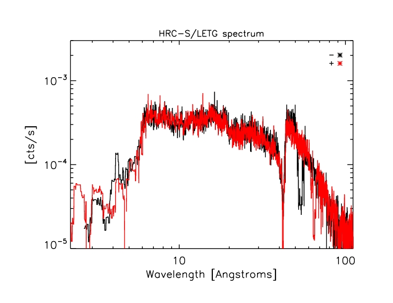
Figure 6: Background-subtracted HRC-S/LETG spectrum of PKS
2155-304 (average of two observations)
The "model" (ie spectrum/ARF):
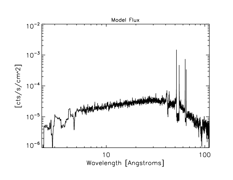
Figure 7: Model derived from HRC-S/LETG spectra
The predicted HRC-I spectrum (model * HRC-I 0th order ARF):
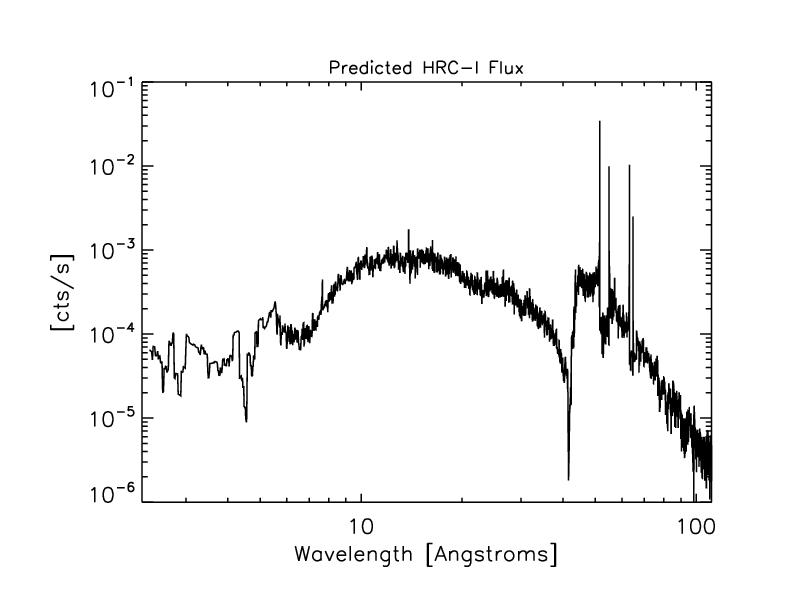
Figure 8: Predicted HRC-I spectrum.
3.2.3 Predicted Rate
We sum the predicted HRC-I spectrum (shown above in Figure 8) over 0.1
- 5.6 keV (where the model is > 0) to get the predicted 0th order
count rate of 1.639 +/- 0.052 cts/s (6.6% higher than the observed
rate) with HRC-I QE model N0007 and 1.669 +/- 0.054 cts/s (8.6% higher
than the observed rate) with model N0007prime.
3.3 Soft Band: HZ 43
3.3.1 Observed HRC-I Count Rates
Count rates are taken from reprocessed level=2 event files which have
been custom filtered to exclude times where the deadtime fraction is
less than 0.985. Source rates are extracted from a circular region
with radius 4.5" and background rates are taken from an annular region
with inner radius 31.6" and outer radius 52.7".
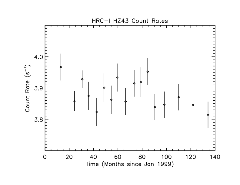
Figure 9: Background-subtracted 0th order count rates for HZ43.
The mean rate is 3.88 cts/s with standard deviation 0.05. The mean of errors is 0.04.
3.3.2 Source Model
As for PKS 2155-304, we construct a source model for HZ 43 using the
HRC-S/LETG observations. For each observation, we smooth source and
background counts from the PHA file (using PoA smoothie, which
conserves flux), subtract the background, then divide the net counts
spectrum by the exposure time and grating ARF. For each observation
this "model" is set to zero where the ARF is less than 0.01 cm^2. The
plus and minus orders are averaged, and finally the observations are
averaged. However, there is a complication for this source: the
observed count-rates have declined by ~9% since the initial
observation due to QE decline in the HRC-S. This decline is apparent
in the following plot of HRC-S/LETG 0th order count rates:
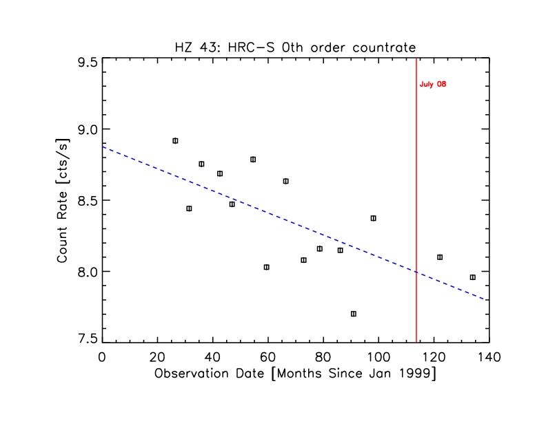
Figure 10: HRC-S/LETG 0th order background-subtracted count
rates with best-fit linear model shown in blue. The red vertical
line marks July 2008, the epoch to which the HRC-S QE model is
pinned.
To compensate for the HRC-S QE decline, we multiply the ARF for each
observation by a corrective factor based on the linear fit to 0th
order count rates (norm=[yint + tnrm*slope]/[yint
+ obs_date*slope] where tnrm corresponds to July 2008)
when constructing the HZ 43 "model".
The combined HRC-S/LETG spectrum:
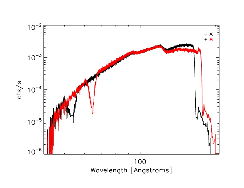
Figure 11: Combined HRC-S/LETG spectrum
The "model" (ie spectrum/ARF):
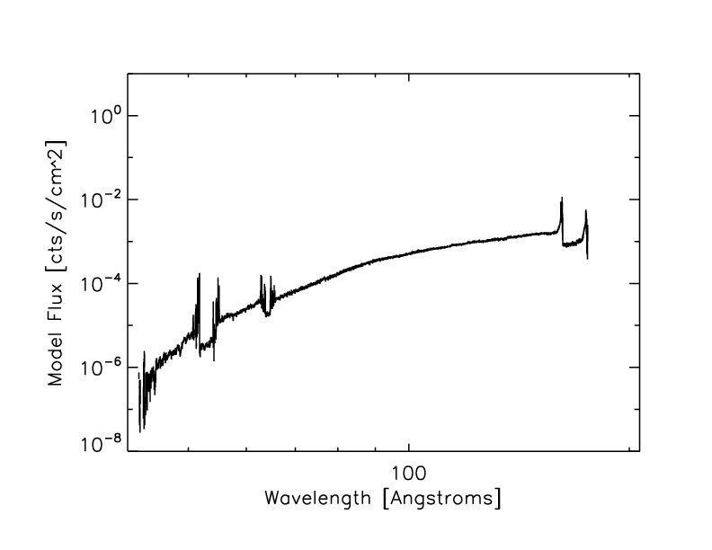
Figure 12: HZ 43 Model
The predicted HRC-I spectrum (model * HRC-I ARF):
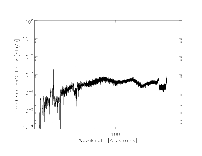
Figure 13: Predicted HRC-I spectrum
3.3.3 Predicted Count Rate
We sum the predicted HRC-I spectrum (shown above in Figure 13) over 0.06 - 0.3 keV to get a
predicted 0th order count rate of 3.46 +/- 0.21 cts/s (10.8% below the
observed rate) with HRC-I QE model N0007 and 4.03 +/- 0.25 cts/s (3.9%
above the observed rate) with model N0007prime.
Table 1: Summary of calibration observations used for QE analysis.
| Source | Instrument | ObsID | Date | Exposure
(s) |
|---|
| G21.5-0.9 | ACIS-S3 | 1553 | 2001-03-18 | 9741.1 |
| 1554 | 2001-07-21 | 9060.7 |
| 3693 | 2003-05-16 | 9783.6 |
| HRC-I | 2867 | 2002-03-12 | 18438.0 |
| 2874 | 2002-07-15 | 19762.4 |
| 3694 | 2003-05-15 | 17055.9 |
| 3701 | 2003-11-09 | 12846.9 |
| 5167 | 2004-03-25 | 18984.0 |
| 6072 | 2005-02-26 | 19018.7 |
| 6742 | 2006-02-21 | 19134.6 |
| 8373 | 2007-05-25 | 19983.5 |
| 10648 | 2009-02-17 | 10054.2 |
| PKS 2155-304 | HRC-S/LETG | 3709 | 2002-11-30 | 13741.8 |
| 4406 | 2002-11-30 | 13762.8 |
| HRC-I/LETG | 3716 | 2002-11-30 | 7328.6 |
| HZ 43 | HRC-S/LETG | 1011 | 2001-03-18 | 18774.9 |
| 1012 | 2001-08-18 | 20807.7 |
| 2584 | 2002-01-01 | 19004.0 |
| 2585 | 2002-07-23 | 19989.8 |
| 3676 | 2002-12-04 | 20716.5 |
| 3677 | 2003-07-24 | 20008.8 |
| 5042 | 2003-12-20 | 21377.1 |
| 5044 | 2004-07-19 | 19693.1 |
| 5957 | 2005-02-02 | 21371.7 |
| 5959 | 2005-07-29 | 18180.1 |
| 6473 | 2006-03-13 | 20901.2 |
| 6475 | 2006-08-07 | 21771.7 |
| 8274 | 2007-03-14 | 20189.3 |
| 10622 | 2009-03-18 | 20292.0 |
| 11933 | 2010-03-15 | 20365.9 |
| HRC-I/LETG | 1514 | 2000-02-03 | 2159.6 |
| 1000 | 2001-01-12 | 3891.8 |
| 1001 | 2001-07-25 | 4955.0 |
| 2600 | 2002-01-02 | 1893.4 |
| 2602 | 2002-07-23 | 1893.3 |
| 3714 | 2003-01-24 | 1868.7 |
| 3715 | 2003-07-24 | 1894.1 |
| 5043 | 2003-12-20 | 1980.8 |
| 5045 | 2004-07-19 | 2145.3 |
| 5958 | 2005-02-20 | 2171.4 |
| 5960 | 2005-08-08 | 1758.9 |
| 6474 | 2006-01-25 | 2154.1 |
| 6476 | 2006-07-24 | 2177.8 |
| 8275 | 2007-03-19 | 2173.7 |
| 9619 | 2008-03-14 | 2164.9 |
| 10623 | 2009-03-11 | 2177.4 |
| 11934 | 2010-03-20 | 2176.0 |
4. Renormalize N0007prime to get new QE, N0008
4.1 Below 0.62 keV
First we renormalize the "re-pasted" section of model N0007prime,
i.e. below 0.62 keV, based on predicted and observed HZ 43 count rates
and on the PKS 2155-304 spectra/ARF ratios for this energy range.
The observed rate for HZ 43 is 3.88 +/- 0.07 cts/s and the predicted rate with N0007prime is 4.03 +/- 0.25, giving a ratio of 1.03866 with uncertainty sqrt((0.25/4.03)^2+(0.07/3.88)^2)*(4.03/3.88) = 0.0671025.
For PKS 2155-304 the ratio of (HRC-I spectrum / HRC-Iprime ARF) to (HRC-S combined spectrum / HRC-S ARF) has mean 0.983 with standard deviation 0.260 in the 20-31 Angstrom range.
(HRC-I spectrum/ARF) / (HRC-S combined spectra / ARF):

Figure 14: Ratio of ARF-corrected HRC spectra for PKS 2155-304.
Close-up of range softwards of the pasting point:
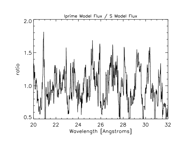
Figure 15: Close-up of ratio of ARF-corrected HRC spectra.
The mean value of the ratio in this range (20-31 Angstroms) is 0.983 with standard deviation 0.260.
The error-weighted mean of the I:S ARF-corrected spectrum ratios is
~1.027. So we divide the HRC-S shifted QE by 1.027 below 0.62 keV, then redo the paste to get model
N0007prime_renorm. Predicted counts with this model are shown in Table 2.
New paste:
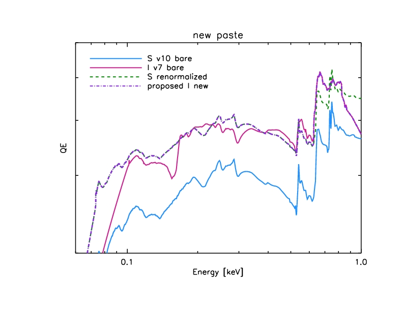
Figure 16: QE paste with correct low-energy normalization.
Closeup: (The pasting point is just below 0.63 keV)
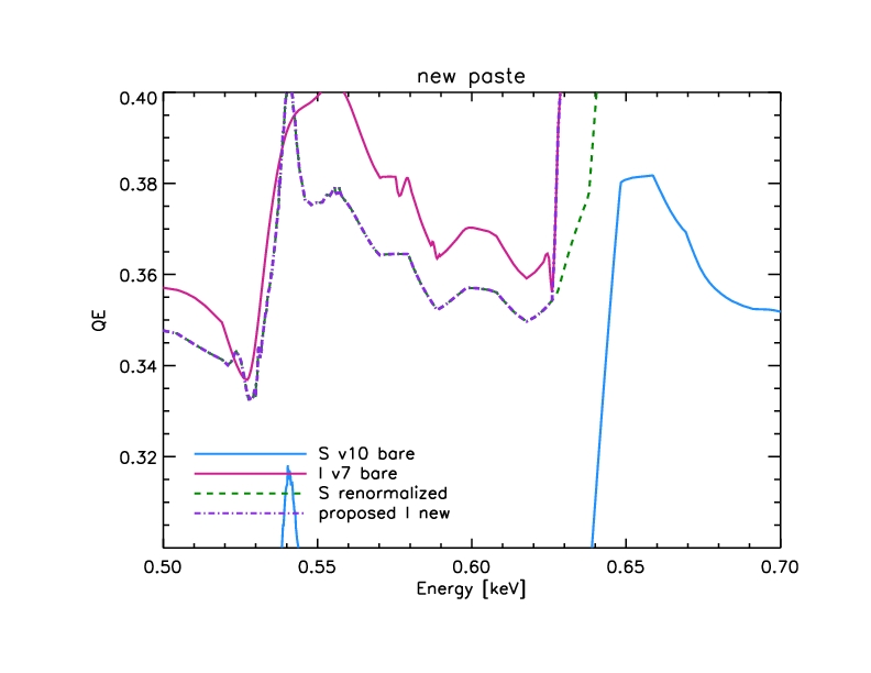
Figure 17: Close-up of QE paste with correct low-energy normalization.
With this new model (N0007prime_renorm) the ratio of I to S
ARF-corrected spectra for PKS 2155-304 has mean 1.01 and standard
deviation 0.267 in the 20-31 Angstrom range.
4.2 Large-scale correction
Finally, we do a large-scale, energy-dependent correction to model
N0007prime_renorm to get the new HRC-I QE model N0008. For the
correction function, we use a step function convolved with a
Gaussian:
f(E)= (K/2) * (1 - Erf[ (E - E_s) / (sqrt(2) * sigma) ] + constant
where
K = amplitude of step function
E_s = energy where step is located
sigma = Gaussian sigma
constant = constant offset
We chose this function since it has the simplicity of a step function
but is continuous to avoid introducing any artificial edges in the QE
model.
We fix sigma to a narrow value of 0.1 keV and constrain the value of the constant so that f(0)=1.
To find values of K and E_s, we do a grid search, computing the
predicted count rates for G21.5-0.9, PKS 2155-304 and HZ 43 for each
pair of values by multiplying f(E) with the source model and ARF (made
with HRC-I QE model N0007prime_renorm). The values yielding the
minimum chi-square (0.25) are E_s = 0.35 keV and K=0.099.
The correction function:

Figure 18: Correction function applied to model
N0007prime_renorm to get model N0008.
We multiply this function with model N0007prime_renorm to get the new
HRC-I QE model N0008.
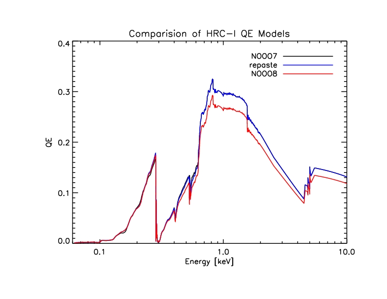
Figure 19: Comparison of HRC-I QE models
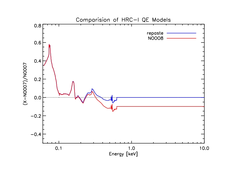
Figure 20: Ratio of new (N0008) and intermediate QE models to
old (N0007) QE model.
5. Summary
We have updated the HRC-I QE model by adjusting the low energy shape and
the global normalization. We use observations of G21.5-0.9, PKS 2155-304
and HZ 43 to cross-calibration with the HRC-S/LETG and ACIS. The mean
squared error (including bias and combined variance from data and model
uncertainties) is given in the last row, signifying the contribution of
calibration uncertainty to predicted count rates. The uncertainty
at low energies is approximately 6%, and at medium and high energies
it is approximately 3%.
The new HRC-I QE model (N0008) was released in the December 2010 CALDB.
Table 2: Summary of observed and predicted count rates
| Source | Observed Count Rate | Predicted Count Rate |
|---|
| with N0007 | with N0007prime | with
N0007prime_renorm | with N0008 |
|---|
| G21.5-0.9 | 0.541+/- 0.008 | 0.601 +/- 0.018
(+9.98% +/- 3.00%)
| 0.601 +/- 0.018
(+9.98% +/- 3.00%) | 0.601 +/- 0.018
(+9.98% +/- 3.00%) | 0.541 +/- 0.016
(0% +/- 2.96%) |
| PKS 2155-304 | 1.537 +/- 0.014 | 1.639 +/-
0.052
(+6.22% +/- 3.17%) | 1.669 +/- 0.054
(+7.91% +/-
3.24%) | 1.644 +/- 0.052
(+6.51% +/- 3.16%) | 1.535 +/-
0.052
(-0.13% +/- 3.39%) |
| HZ 43 | 3.88 +/- 0.07 | 3.46 +/- 0.21
(-12.50% +/-
6.07%) | 4.03
+/- 0.25
(+3.72% +/- 6.20%) | 3.92 +/- 0.24
(+1.02% +/-
6.12%) | 3.91 +/- 0.24
(+0.77% +/- 6.14%) |
| MSE | 0.243 | 0.114 | 0.087 | 0.066 |
Appendix: Checking the cross calibration with E0102
To check the HRC-I / ACIS-S cross calibration, we use observations of
the supernova remnant 1E0102-72.3 ("E0102"). E0102 has been observed twice with
the HRC-I, in Oct 1999 and Mar 2010, and numerous times with ACIS over
the course of the Chandra mission. Note that this calibration source
was not used in the construction of the N0008 or preceding HRC-I QE models.
From the two HRC-I observations, we get background-subtracted source
count rates of 3.22 +/- 0.01 cts/s (ObsID 1410, 1999-10-25) and 3.20 +/-
0.01 cts/s (ObsID 11093, 2010-03-04). The errors given are 1 sigma.
To calculate a predicted count rate for the HRC-I, we use as a
source model a joint fit to two ACIS-S3 subarray observations (ObsIDs
3545 and 6765) with the IACHEC E0102 model. (See the Plucinsky
et al 2008 SPIE paper for more information about this model.) The
ACIS data are fit between 0.3 - 2 keV and the ACIS ARF includes
contamination model N0007. The ACIS spectra and HRC-I counts are
extracted from a circular region with radius 25.3" centered at J2000
coordinates (R.A.,
Dec.) = (01:04:01.996, -72:01:53.44).
From this source model and an HRC-I ARF (using HRC-I QE model N0008),
we get a predicted count rate of 3.16 +/- 0.01 cts/s. The
uncertainty on the predicted rate is taken from the standard deviation
of 5000 MCMC iterations, sampling among the errors on the free
parameters in the ACIS fit.
Last modified:
05/23/18