[Last Change: 25 Apr 2012 (rev 23) — Page History]

How to raytrace a dithered observation

Overview

SAOTrace can simulate the telescope motion during an observation in two ways:

1. It can read an existing aspect solution file
2. It can directly generate ideal Lissajous dither motions.

Unfortunately the internal dither generate is not of much practical use for the observer, as there is currently no way of generating a related aspect solution file which can be used to correct for this motion and generate a level 2 event file.

Using an aspect solutions file

Aspect solution files provide the absolute orientation of the spacecraft relative to the celestial sphere as it varies through an observation. Every Chandra observation has an aspect solution file associated with it. It is also possible to generate aspect solution files with MARX (which can be useful when simulating observations for proposal purposes or for Monte Carlo analyses of existing observations).

SAOTrace can use either Chandra aspect solution files or MARX generated aspect solution files. To use a Chandra aspect solution file, add the following to your trace-nest source parameters:

dither_asol_chandra{ file = asolfile, ra = RA_PNT, dec = DEC_PNT, roll = ROLL_PNT }

Where asolfile is the path to the observation's asol1 file, and RA_PNT, DEC_PNT, and ROLL_PNT are the values of the similary named header keywords in the observation's level 2 event file. For a very few observations these keywords are available only in the level 1 events file. The values may be extracted with the CIAO dmkeypar command.

To use a MARX generated aspect file, add the following:

dither_asol_marx{ file = asolfile, ra = RA_PNT, dec = DEC_PNT, roll = ROLL_PNT }

Where asolfile is the path to the MARX generated aspect solution file, and RA_PNT, DEC_PNT, and ROLL_PNT are as described above.

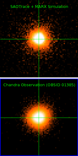
Example Simulation of OBSID 1385

OBSID 1385 is an HRC-I observation of AR Lac. We'll use MARX (version 5) to simulate the detector. MARX requires source and pointing positions to be specified in degrees.

The following data are required

• The telescope pointing in celestial coordinates and the telescope roll
• The position of the object in celestial coordinates
• The observation starting time and exposure duration

Telescope Point and Roll

The pointing and roll values are extracted with the CIAO dmkeypar command from the Chandra level 2 event file:

% dmkeypar hrcf01385_evt2.fits.gz RA_PNT echo+
332.16395709286

% dmkeypar hrcf01385_evt2.fits.gz DEC_PNT echo+
45.740257117459

% dmkeypar hrcf01385_evt2.fits.gz ROLL_PNT echo+
230.44376969211

Celestial Source Position

The source position has been determined from the existing Chandra observation as

RA	Dec
22:08:40.829	+45:44:32.56
332.170120833333	45.7423777777778

Start time and Exposure Time

We'll also need the start time and an exposure time. We would like to use the actual science data start time, i.e. the time at which the telescope has reached a stable position after slewing to the target, but due to current limitations in software, that may not be possible, so it's important to understand which times are appropriate.

Simulations using MARX

The current version of MARX (5.0.0) which can accept dithered rays from SAOTrace uses the TSTART and TSTOP times stored in the headers of the Chandra aspect solution file to determine the beginning and duration of the simulation. Unfortunately, this period includes data taken during telescope slew, and so the event file output by MARX must be GTI filtered.

The TSTART and TSTOP quantities may be extracted from the Chandra aspect solutions file with dmkeypar:

% dmkeypar primary/pcadf055469783N003_asol1.fits.gz tstart echo+
55469783.7854612

% dmkeypar primary/pcadf055469783N003_asol1.fits.gz tstop echo+
55488887.9923994


# calculate the total exposure time
% perl -le 'print 55488887.9923994 - 55469783.7854612'
19104.2069381997

which gives

Start time	= 55469783.7854612
Exposure time	= 19104.2069381997

Simulations not using MARX

If not using MARX, one can use the actual start and stop of science data time, which is most easily determined from the level 2 event file's GTI records:

% dmlist hrcf01385_evt2.fits.gz'[GTI]' data

--------------------------------------------------------------------------------
Data for Table Block GTI
--------------------------------------------------------------------------------

ROW    START                STOP

     1  55469832.9854629636  55469982.6354683563
     2  55470017.4854696095  55470018.5104696453
     3  55470055.4104709774  55470784.1854970008
     4  55470786.2354969978  55472780.8855689988
     5  55472782.9355690032  55479418.7858079970
     6  55479420.8358080015  55486056.6860470027
     7  55486058.7360479981  55488887.9923994020

% perl -le 'print 55488887.9923994020 - 55469832.9854629636'
19055.0069364384

This gives

Start time	= 55469832.9854629636
Exposure time	= 19055.0069364384

Running a raytrace

The trace-nest source definition (in the file 01385.lua) is:

ra_pnt   = 332.16395709286
dec_pnt  = 45.740257117459
roll_pnt = 230.44376969211

dither_asol{ file = 'pcadf055469783N003_asol1.fits.gz',
        ra   = ra_pnt,
        dec  = dec_pnt,
        roll = roll_pnt
        }
point{ position = { ra = '22:08:40.829',
          dec = '+45:44:32.56',
          ra_aimpt = ra_pnt,
          dec_aimpt = dec_pnt,
       },
       spectrum = { { 1.49, 0.01 } }
    }

In this example we'll be sending the resultant rays into MARX, so we'll use the start time and exposure time derived from TSTART and TSTOP.

To run the raytrace, issue the following command (after setting the default parameters):

trace-nest                    \
   tag=01385                  \
   srcpars=01385.lua          \
   tstart=55469783.7854612   \
   limit=19104.2069381997    \
   limit_type=sec

To the right is an image of the simulated rays prior to running through MARX.

Now to run MARX.

MARX requires the Chandra aspect solution file, but it does not read compressed FITS files, so first decompress the aspect solution file:

gunzip pcadf055469783N003_asol1.fits.gz

Then, set the MARX parameters using pset. It's important to keep the MARX parameter file up-to-date as the marx2fits program reads parameters from it.

pset marx \
    DetectorType=HRC-I               \
    GratingType=NONE                 \
    SourceType=SAOSAC                \
    SAOSACFile=01385.fits            \
    SourceRA=332.170120833333        \
    SourceDEC=45.7423777777778       \
    RA_Nom=332.16395709286           \
    Dec_Nom=45.740257117459          \
    Roll_Nom=230.44376969211         \
    TStart=55469783.785461           \
    ExposureTime=19104.2069381997    \
    OutputDir=01385                  \
    DitherModel=FILE                 \
    DitherFile=pcadf055469783N003_asol1.fits

Next, run MARX and convert the results into a Chandra Level 1 event file and then filter the results with the GTI data in the event file using dmcopy

marx

marx2fits 01385 01385-marx.fits
dmcopy "01385-marx.fits[@hrcf01385_evt2.fits.gz[GTI]]" 01385-marx-filtered.fits