| PREVIOUS | INDEX | NEXT |
| Wavelength range | 1.2-175 Å (HRC-S) |
| 1.2-60 Å (ACIS-S) | |
| Energy range | 70-10000 eV (HRC-S) |
| 200-10000 eV (ACIS-S) | |
| Resolution (∆λ, FWHM) | 0.05 Å |
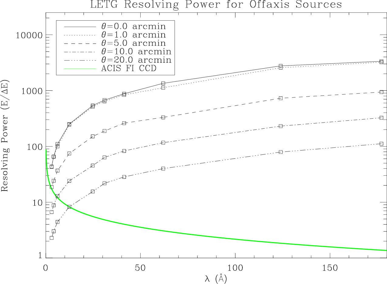
| Resolving Power (λ/∆λ) | ≥ 1000 (50-160 Å) |
| ≈ 20×λ (3-50 Å) | |
| Dispersion | 1.148 Å/mm |
| Plate scale | 48.82 μm/arcsec |
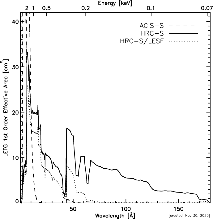
| Effective area (1st order) | 1-25 cm2 (with HRC-S) |
| 1-100 cm2 (with ACIS-S) | |
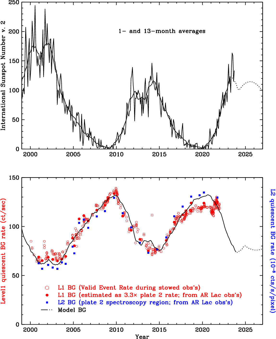
| Background (quiescent) | LETG/HRC-S: 26 (90) cts/0.07-Å/100-ks @ 50 (175) Å |
| for typical L2 background rate (0.10 cts/pixel/100-ks; see Figure 9.21) | |
| LETG/ACIS-S: << 0.01 cts/pixel/100-ks (order sorted) | |
| Detector angular size | 3.37' × 101' (HRC-S; standard 6-tap-wide spectroscopy region) |
| 8.3' × 50.6' (ACIS-S; full 6-chip array) | |
| Pixel size | 6.43 × 6.43 μm (HRC-S) |
| 24.0 × 24.0 μm (ACIS-S) | |
| Temporal resolution | 16 μsec (HRC-S in Imaging Mode, center segment only) |
| ∼ 10 msec (HRC-S in default mode) | |
| 2.85 msec-3.24 sec (ACIS-S, depending on mode) | |
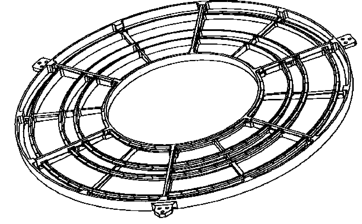
| Rowland diameter | 8637 mm (effective value) |
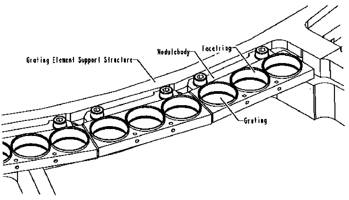
| Grating material | gold |
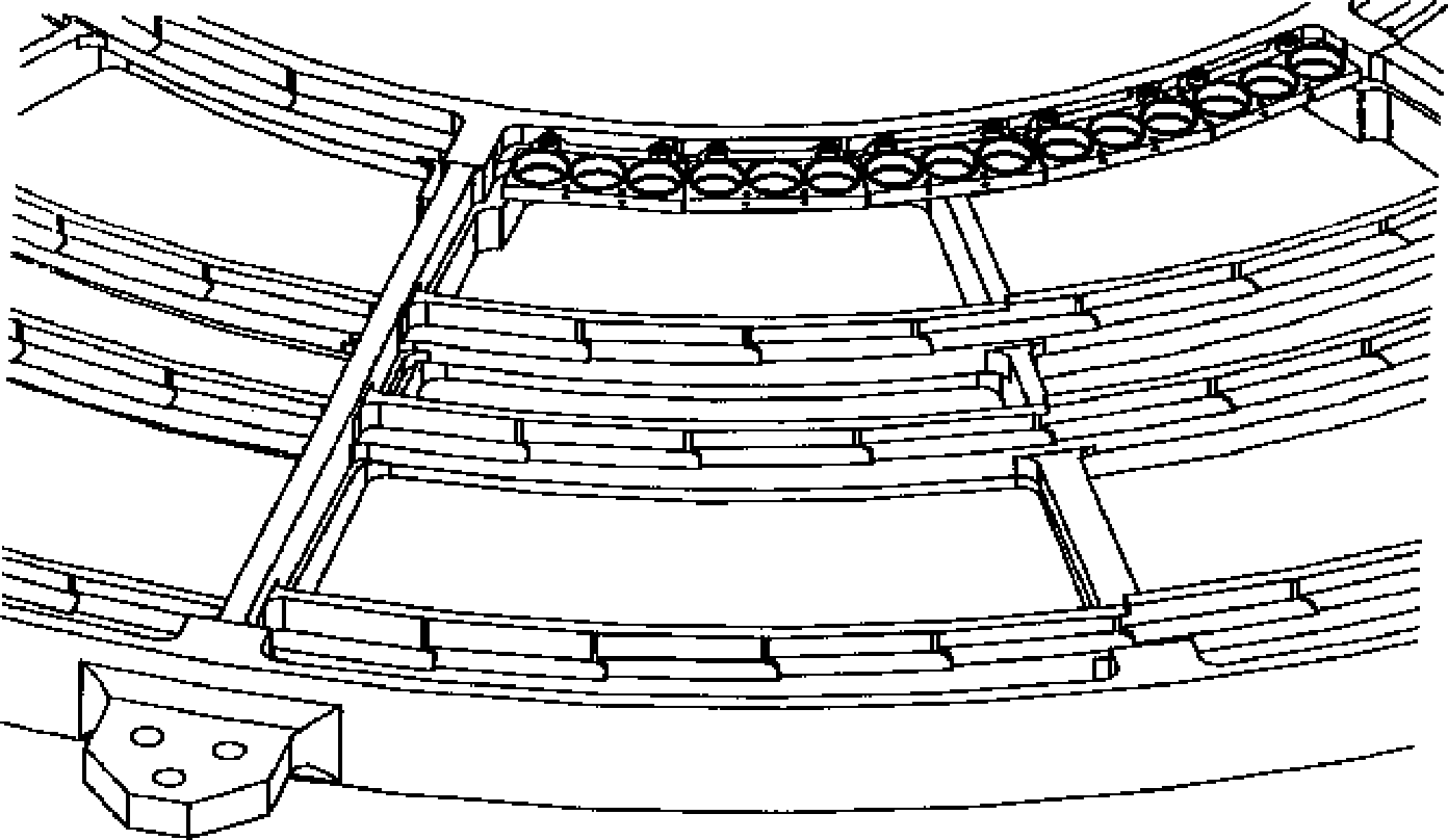
| Facet frame material | stainless steel |
| Module material | aluminum |
| LETG grating parameters | |
| Period | 0.991216 ±0.000087 μm |
| Thickness | 0.474 ±0.0305 μm |
| Width (at bar middle) | 0.516 ±0.0188 μm |
| Bar Shape | symmetric trapezoid |
| Bar Side Slope | 83.8 ±2.27 deg |
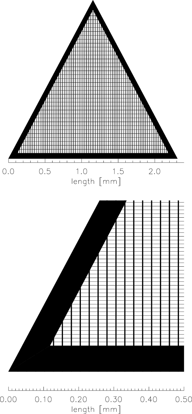
| Fine-support structure | |
| Period | 25.4 μm |
| Thickness | 2.5 μm |
| Obscuration | < 10% |
| Dispersion | 29.4 Å/mm |
| Material | gold |
| Coarse-support structure | |
| Triangular height | 2000 μm |
| Width | 68 μm |
| Thickness | < 30 μm |
| Obscuration | < 10% |
| Dispersion | 2320 Å/mm |
| Material | gold |
| Target | Freq. | Purpose |
| (yr−1) | ||
| Capella | 1 | LETG/HRC-S LRF, dispersion relation, QE, EA |
| PKS 2155-304 | 1 | LETG/ACIS-S EA, ACIS-S contam, cross calib with XMM, Suzaku |
| Mkn 421 | 1 | LETG/ACIS-S and LETG/HRC-S EA, ACIS-S contam, HRC-S gain |
| RX J1856-3754 | 1 | LETG/ACIS-S EA and ACIS-S contam |
| HZ 43 | 1 | LETG/HRC-S EA and HRC-S gain |
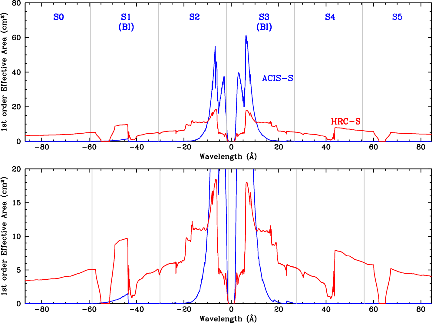
| Detector | Section | Energy | Wavelength |
| (eV) | (Å) | ||
| HRC-S | UVIS Inner T (thick Al) | (650) - 730 | (19) - 17 |
| HRC-S | seg-1 (neg. mλ) | (75) - (221) | (164) - (56) |
| HRC-S | seg0 | (245) - 203 | (50) - 61 |
| HRC-S | seg+1 (pos. mλ) | 188 - 71 | 66 - 175 |
| ACIS-S | S0 (neg. mλ) | (141) - (207) | (87.9) - (59.7) |
| ACIS-S | S1 (Back-illuminated) | (210) - (400) | (59.2) - (31.0) |
| ACIS-S | S2 | (407) - (5300) | (30.4) - (2.3) |
| ACIS-S | S3 (Back-illuminated) | (7300) - 469 | (1.7) - 26.4 |
| ACIS-S | S4 | 460 - 225 | 27.0 - 55.1 |
| ACIS-S | S5 (pos. mλ) | 223 - 148 | 55.7 - 83.8 |

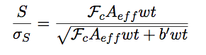
 |
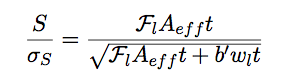
(9.1) |


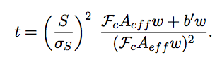
 |
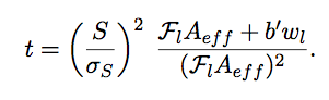
(9.2) |
| Instrument | Element | Edge | Energy | Wavelength |
| (keV) | (Å) | |||
| HRC | Cs | L | 5.714 | 2.170 |
| HRC | Cs | L | 5.359 | 2.313 |
| HRC | I | L | 5.188 | 2.390 |
| HRC | Cs | L | 5.012 | 2.474 |
| HRC | I | L | 4.852 | 2.555 |
| HRC | I | L | 4.557 | 2.721 |
| LETG | Au | M | 3.425 | 3.620 |
| LETG | Au | M | 3.148 | 3.938 |
| HRMA | Ir | M | 2.909 | 4.262 |
| LETG | Au | M | 2.743 | 4.520 |
| HRMA | Ir | M | 2.550 | 4.862 |
| LETG | Au | M | 2.247 | 5.518 |
| LETG | Au | M | 2.230 | 5.560 |
| HRMA | Ir | M | 2.156 | 5.750 |
| HRMA | Ir | M | 2.089 | 5.935 |
| ACIS | Si | K | 1.839 | 6.742 |
| HRC, ACIS | Al | K | 1.559 | 7.953 |
| HRC | Cs | M | 1.211 | 10.24 |
| HRC | I | M | 1.072 | 11.56 |
| HRC | Cs | M | 1.071 | 11.58 |
| HRC | Cs | M | 1.003 | 12.36 |
| HRC | I | M | 0.931 | 13.32 |
| HRC | I | M | 0.875 | 14.17 |
| HRC | Cs | M | 0.7405 | 16.74 |
| HRC | Cs | M | 0.7266 | 17.06 |
| ACIS | F | K | 0.687 | 18.05 |
| HRC | I | M | 0.6308 | 19.65 |
| HRC | I | M | 0.6193 | 20.02 |
| HRC,ACIS | O | K | 0.532 | 23.30 |
| HRMA | Ir | N | 0.496 | 25.0 |
| HRC | N | K | 0.407 | 30.5 |
| HRC,ACIS | C | K | 0.284 | 43.6 |
| HRC | Al | L | 0.073 | 170 |
 |
(9.3) |
 |
(9.4) |
 |
(9.5) |
 |
(9.6) |
 |
(9.7) |
 |
(9.8) |
 |
(9.9) |
 |
(9.10) |
 |
(9.11) |
 |
(9.12) |

| PREVIOUS | INDEX | NEXT |