CalDB 4.5.9 Public Release Notes
Public Release Date: 19 Nov 2013
SDP Installation Date: 2013-11-19T23:25:07 (UTC)
I. INTRODUCTION
CalDB 4.5.9 is an upgrade to the Chandra CalDB, which includes the following items:
- ACIS T_GAIN Epoch 55 (August-October 2013)
- ACIS CONTAM Version N0008
- HRC-I GMAP & PIBGSPEC September 2013
For the CIAO 4.5 / CalDB 4.5.9 release notes see How CalDB 4.5.9 Affects Your Analysis.
II. SUMMARY OF CHANGES
A. ACIS T_GAIN Epoch 55 (August-October 2013)
| Location: | $CALDB/data/chandra/acis/t_gain/ |
| Filename: | acisD2013-05-01t_gainN0005.fits acisD2013-05-01t_gainN0006.fits acisD2013-08-01t_gainN0002.fits acisD2013-08-01t_gain_biN0002.fits |
The periodic ACIS T_GAIN correction upgrade for August-October 2013 (Epoch 55) has been released. The corrections are at nominal/expected levels of less than 2% of the energy value. This upgrade as usual affects observation data taken over the two most recent T_GAIN Epochs (55 and 54), and so would update PHAs for OBS_IDs taken since 01 May 2013. Users with such datasets are encouraged to revalidate their analysis results after reprocessing their data with the upgraded CalDB files. For specific details of the new calibrations in this release, see the technical details section below.
See the ACIS T_GAIN why page for more information.
PIPELINES/TOOLS AFFECTED:
DS and CIAO level 1 (re)processing tool acis_process_events
Also: CIAO reprocessing script chandra_repro
THREADS AFFECTED:
Reprocessing Data to Create a New L2 Events File
B. ACIS CONTAM Version N0008
| Location: | $CALDB/data/chandra/acis/contam/ |
| Filename: | acisD1999-08-13contamN0008.fits |
The ACIS Optical Blocking Filter (OBF) contaminant calibration file requires an update due to recent changes the depth and composition of the contaminant with time. New modeling results from cosmic sources galaxy cluster Abell 1795 and blazar MKN421, in conjunction with fits of SNR EO1O2-72 calibration observations have resulted in a new ACIS contamination model.
The rate of deposition has increased markedly since mid 2009; The cause of this is not certain. However, the shape of deposition curve since 2009 has recently shown a more linear behaviour with time than was previously included in the most recently released CONTAM file model (version N0007, May 2012, CalDB 4.4.10.)
Regarding composition, it appears that the concentration of the several component elements in the contamination layer are also changing, which requires time-varying adjustment of the optical depths for carbon (C-K) and fluorine (F-K) with respect to oxygen (O-K), and a modified spatial model for ACIS-S in particular. A purely elemental model with the appropriate time- and spatially-dependent adjustments has recently been derived, and is being released here.
Caveat to users: Beware when using high ChipY locations on ACIS-S3 for imaging spectroscopy with the CONTAM N0008 model! We are somewhat uncertain of the contaminant layer depth at high chipy for ACIS-S, and fitting results may be compromised at this location. For technical details, see Section II.B. below.
See the ACIS contamination why page for more information general information on the ACIS time-varying QE/OBF contaminant.
PIPELINES/TOOLS AFFECTED:
The following CIAO tools automatically apply the CONTAM correction creating ACIS responses:
The following scripts make use of the above tools, and hence also apply CONTAM:
- specextract (calls mkarf and mkwarf)
- fullgarf (calls mkgarf)
- specextract (calls mkinstmap)
- merge_obs (calls mkinstmap)
THREADS AFFECTED:
Imaging spectroscopy:
- Calculating the ARfs (for pointlike sources)
- Calculating the ARfs (for extended sources)
- Calculating the ARfs (multiple sources)
Grating spectroscopy:
C. HRC-I GMAP & PIBGSPEC September 2013
| Location: | $CALDB/data/chandra/hrc/gmap/ |
| Filename: | hrciD2013-09-16sampgainN0001.fits |
| Location: | $CALDB/data/chandra/hrc/pibgspec/ |
| Filename: | hrciD2013-09-16pibgspecN0001.fits |
The annual update to the HRC-I time-dependent gain and the corresponding PI Background Spectrum are now available. Technical DETAILS of the new GMAP image are available below.
See the HRC-I Gain Maps why page for more information.
PIPELINES/TOOLS AFFECTED:
GMAP only: hrc_process_events
THREADS AFFECTED:
For the GMAP: Reprocessing Data to Create a New Level=2 Event File
For the PIBGSPEC: The HRC-I Background Spectra Files
III. TECHNICAL DETAILS
A. ACIS T_GAIN Epoch 55 (August-October 2013)
The ACIS time-dependent gain corrections (T_GAIN) have recently been updated for current changes from the previous T_GAIN epoch, specifically Epoch 55, which was August-October 2013. With the addition of these new corrections, derived from ACIS External Cal Source (ECS) data taken during radiation zone passes, the CalDB files extending from May-August 2013 (i.e. Epoch 54) have been finalized, and new non-interpolating T_GAIN files are now implemented for Epoch 55.
The magnitudes (in eV) of the new gain corrections, versus photon energy, are given in Figs. 1-3 below. The corrections are of the usual order in magnitude, specifically less than 2.0% of the photon energy value. Fig. 1 below gives the corrections for the ACIS-I aimpoint on chip ACIS-3, for the CTI-corrected case, which is the only one applicable to FI chips. Figure 2 gives the corrections for the ACIS-S aimpoint on ACIS-7, for the case where the BI chips are CTI-corrected. Finally Fig. 3 gives the corrections for ACIS-7 for NON-CTI-corrected BI chips. These would be relevant to GRADED DATAMODE observations with ACIS-S, for example.
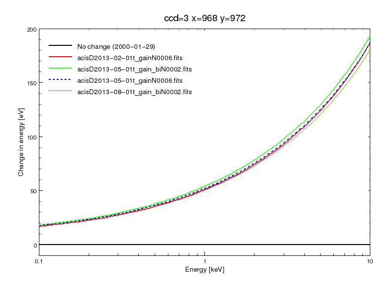
Fig. 1: ACIS-I3 aimpoint T_GAIN corrections in eV versus photon energy.
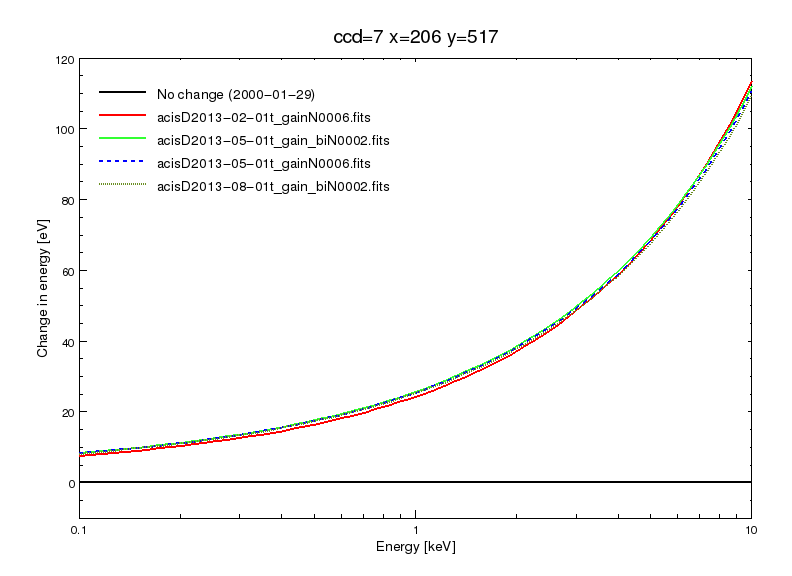
Fig. 2: ACIS-S3 CTI-corrected aimpoint T_GAIN corrections in eV versus photon energy.

Fig. 3: ACIS-S3 non-CTI-corrected aimpoint T_GAIN corrections in eV versus photon energy.
Long term trends for chips I3 and S3 are plotted below in Figure 4a and b, through Epoch 55, the latest release. The chip locations for these plots are given in the respective labels above the plots. Note that the locations are not the aimpoint positions, as with Figs. 1-3 above, but are near the centers of each chip.
|

|
| Figs 4a and 4b: Long term gain trends for specific ECS line energies from Epoch 1 to Epoch 55 inclusive, and for the positions on the respective chips given in the figure labels. (Click on images to expand the plots.) | |
B. ACIS CONTAM Version N0008
The deposition rate and composition of the contaminating layer on the ACIS Optical Blocking Filter (OBF) continues to change and require adjustments to the model used to estimate its absorption effects. With this new N0008 release, for the first time there is a systematic, purely elemental model (no edgeless "fluffium" component) for the ACIS contamination. This has been made possible by varying not only the depth, but the chemical composition of the contaminant with time and location.
Figure 5 below gives the estimated optical depth (tau) of the contaminant versus mission date. Note the change in the deposition rates throughout the mission, and in particular the abruptly upward, almost linear, increase in the contamination rate beginning in mid 2009. Fig. 6 gives the change in tau between the center and the edge of the detector, which shows that the increasing spatial variation of the contaminant with time.
Fig. 5: The optical depth "tau" of the contaminating layer on the ACIS OBF as modeled versus year of the mission time line. Note that the trend since y2009 has been essentially a linear increase with time. |
Fig. 6: This figure shows that difference in the optical depth at 700 eV between the edge and center of the detector. |
Fig. 7 below shows the accumulation rates for carbon and oxygen. In particular for the period 2003-2005, the composition of the contaminant appears to have been changing with time.
Fig. 7: The Carbon and Oxygen deposition rates versus year, showing the
variation in the composition of the contaminating layer.
While the most recent (2013) data taken to monitor the contaminating layer indicate the layer depth is almost linearly increasing with time since 2009, the previous model (N0007) anticipates a leveling-off of the contamination layer going forward. Hence a new model is needed properly to account for the current trend. Upgrading the model for the full mission means that the new CONTAM model is not identically backward compatible with the previous version (N0007, released in CalDB 4.4.10, May 2012). However, the new model fits the tau for all periods illustrated in Figs 5 and 6 above, and hence does not significantly affect midmission results.
This is the procedure that has been employed in developing the new contamination model:
- Develop a preliminary contamination model to fit Abell 1795 data at the centers of both ACIS-I and ACIS-S arrays as a function of time. Add a spatial component appropriate for each array.
- Using the preliminary model, fit LETG/ACIS-S spectra of blazars to constrain the optical depths at the C-K, O-K, and F-K edges. The gratings data is primarily restricted to two rows (167 and 32) on ACIS-S. (Fig. 8 below.)
- Fit the raster scans of Abell 1795 observations using a purely elemental model, adopting edge constraints measured from the gratings data, and determine the normalization of the contamination model as a function of position and time.
- Make final adjustments in tau(C-K) and tau(F-K) as a function of TIME, using LETG/ACIS-S data. No adjustment is needed at the O-K edge. (Result: The new CalDB CONTAM file N0008)
- Verify the model by fitting E0102-72 observations at various locations on ACIS-I3 and ACIS-S3, using the Standard IACHEC E0102 Model. (See Fig 9a-f below.)

Fig. 8: The C-K optical depth determined from fits of blazar gratings data
using a preliminary contamination model (designated 9951) for ACIS-S.
Hence, ACIS CONTAM version N0008 accomplishes two goals, (1) implementation of a more realistic model (without the edgeless "fluffium" component used in previous models) and (2) more accurate representation and prediction of current and future loss of effective ACIS QE due to the OBF contamination layer.
Fitting spectra from E0102-72 taken at various times during the mission (on ACIS-I and ACIS-S) indicates that the CONTAM N0008 model is basically successful (Fig. 9a-f below.) However, we note that there is one particular position on ACIS-S3 where the E0102-72 certain line normalizations are skewed with respect to the general results, specifically in the high ChipY location of Node 2. (See the green square symbol in each of Fig. 9b, c, and d.)
Caveat to users: Beware when using high ChipY locations on ACIS-S3 for imaging spectroscopy with the CONTAM N0008 model! We are somewhat uncertain of the contaminant layer depth at high chipy for ACIS-S, and fitting results may be compromised at this location.
Fig. 9a: Fitting E0102-72 on ACIS-S3 with the standard IACHEC model and CONTAM N0008: Overall Normalization. |
Fig. 9b: Fitting E0102-72 on ACIS-S3 with the standard IACHEC model and CONTAM N0008: O-VII Normalization. |
Fig. 9c: Fitting E0102-72 on ACIS-S3 with the standard IACHEC model and CONTAM N0008: O-VIII Normalization. |
Fig. 9d: Fitting E0102-72 on ACIS-S3 with the standard IACHEC model and CONTAM N0008: Ne-IX Normalization. |

Fig. 9e: Fitting E0102-72 on ACIS-S3 with the standard IACHEC model and CONTAM N0008: Ne-X Normalization. |
Fig. 9f: Fitting E0102-72 on ACIS-S3 with the standard IACHEC model and CONTAM N0008: Goodness of fit. |
The overall affect of the increasing contamination layer is best illustrated using spectra from Abell 1795, a stable source observed by the ACIS Calibration team annually since the start of the mission. See Fig. 10, for an illustration of the loss of effective ACIS-S effective area with time. These data have been used for the first step in modeling the contaminant layer with time.
Fig. 10: This figure shows the result of a simultaneous
fit to spectra extracted from nine observations of A1759 in 2000, 2002, 2004,
2005, 2009, 2010, 2011,2012 and 2013.
The comparative ACIS-I effective areas (EAs) for January 01 of 2000, 2004, 2009, and projected for 2015, are given in Fig. 11 below. The solid curves are those calculated using CONTAM N0007; the dashed curves of the corresponding color are for the same dates, but using the new CONTAM N0008 file. The early- and mid-mission EAs are not much affected by the new model, except for very near the C-K, O-K, and F-K absorption edges, as would be expected from the new elemental basis of the model. (Changes near these edges do not affect users' fitting results significantly for mid-mission observations.)
Fig. 11: The ACIS-I aimpoint effective areas versus Energy for January 01 of 2000 (green),
2004 (blue), 2009 (cyan), and projected for 2015 (red). The solid curves give the calculation
using CONTAM N0007; the dashed curves give the same, but using CONTAM N0008.
The comparative ACIS-S effective areas (EAs) for January 01 of 2000, 2004, 2009, and projected for 2015, are given in Fig. 12 below. The solid curves are those calculated using CONTAM N0007; the dashed curves of the corresponding color are for the same dates, but using the new CONTAM N0008 file. The early- and mid-mission EAs are not much affected by the new model, except for very near the C-K, O-K, and F-K absorption edges, as would be expected from the new elemental basis of the model. (Changes near these edges do not affect users' fitting results significantly for mid-mission observations.)
Fig. 12: The ACIS-S aimpoint effective areas versus Energy for January 01 of 2000 (green),
2004 (blue), 2009 (cyan), and projected for 2015 (red). The solid curves give the calculation
using CONTAM N0007; the dashed curves give the same, but using CONTAM N0008.
However, the more rapidly increasing contamination layer does indicate that ACIS-S is not optimal for very soft sources in the future, particularly at and below the Carbon edge (283 eV). It is suggested that LETG/HRC-S is a better configuration in this energy range going forward, with larger EAs and better calibrations as well.
C. HRC-I GMAP & PIBGSPEC September 2013
A new HRC-I GMAP has been generated for the (UTC) period 2013-09-16T12:00 to the present, and extending into 2014. The corrections were generated using G21.5-0.9 and HZ 43 calibration observations taken regularly to monitor HRC-I, combined with a sequence of ArLac observations at 21 specific locations on HRC-I, taken annually.
The HRC-I gain continues to decline slowly (typically ≤5% per year). Annual updates to the gain maps are found to be adequate to maintain 2% consistency in the PI. Images of the new Sept 2013 GMAP, and a ratio of the new map to the previous (2012) one already in CalDB are shown in Fig. 13A & B below. In Fig. 13B, the sense of the ratio is that the 2013 map includes equal to or larger corrections (equal to or greater than unity) compared with last year's gmap.

Fig. 13A: The new HRC-I GMAP derived from Sept 2013 ArLac observations, and periodic HZ43 and G21.5-0.9 observations. |
Fig. 13B: Ratio of the new 2013 GMAP to the one from 2012. |
A corresponding upgrade to the PIBGSPEC library fo 2013 has also been derived, effective for the same time-period as the above HRC-I GMAP. The background PI spectra are generated from the same HRC-I calibration observations of AR Lac used to derive the new GMAP. These 21 observations are reprocessed with the new GMAP, generating new PI scaled to SUMAMPS values.
For each year, the HRC-I Cal team extracts events in a 800x800 pixel box at the 17 observation locations that are within 10 arcmin of the aim point, excluding the location of the source. They sum the PI spectra from each location, weighting by exposure time, to create the final PI spectrum for the year. Finally, the PI spectra are Loess-smoothed with a third-degree polynomial fit over ranges 10 channels wide.
Figure 14 shows the PI spectra (as calculated count rates) for several of the PIBGSPEC files from 2000 (black), 2005 (red), 2009 (green), 2010 (blue), 2011 (cyan), 2012 (magenta), and 2013 (yellow):
Fig. 14: The HRC-I Background PI spectra for 2000-2013, including the latest
spectrum derived from Sept 2013 AR Lac data.