Investigating Colors of Variable Galactic Sources
CSC Threads
Overview
Synopsis:
Last Update: 16 Sep 2013 - Initial version.
Contents
Science question
Is there a relationship between variability and spectral color for Galactic sources? If so, then possibly a new type of classification scheme can be created to predict an object's type based on these two parameters.
In X-ray astronomy, colors are represented as a hardness ratio. The two terms are used here interchangeably. The CSC has data available for 3 different hardness ratios: ACIS hard band to soft band, hard band to medium band, and medium band to soft band. Each are normalized by the broad band flux.
Creating the CSCView query
Select which sources to include
This search begins with an empty search form. In the CSCView go to File → New → Empty Form. Since the question being asked requires only galactic sources, the search begins by selecting the gal_b, galactic latitude, from the Master Sources → Source Position → Galactic Coordinates list and adding it to the Search Criteria. For this investigation, the galactic plane is taken to mean |gal_b|<20. The query could be constructed by using gal_b > -20 AND gal_b < 20 ; however, the ADQL syntax allows for a BETWEEN operator as is shown in Figure 1.
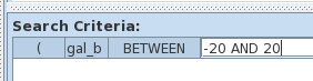
Figure 1: Restricting the search to just galactic sources with latitude between -20 and 20 degrees.
The HRC instrument does not have sufficient energy resolution to determine colors, so the search is further constrained to just include data obtained with ACIS. The instrument is selected from the Source Observations → Observation-Specific Information → Instrument Configuration list.

Figure 2: Select only ACIS observations.
Note that this query combines properties from the Master Sources table and the Source Observation table. CSCView will automatically extend the query to include the linkage between these without requiring anything more from the user.
These are the only search criteria that will be used. The analysis that will be conducted will compare the hardness ratios of variable sources to non-variable sources, where the definition of variable is one of the parameters to be examined.
Select which columns to return
If the search of variable sources yields some interesting subclass of sources, then being able to track them back to the original dataset will require knowing the source name, the observation identifier, obsid with obi number, and the region_id. These are added to the Result Set as in Figure 3.
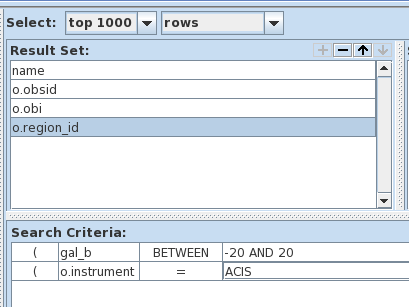
Figure 3: Columns required to trace source back to original per-observation source.
Next the ACIS broad band variability columns are added (Figure 4) along with the spectral colors or hardness ratio values (Figure 5). All the columns for these two class of properties are added; the analysis will select from them later. They can either be selected individually, or the entire group can be added at once by selecting the group name.
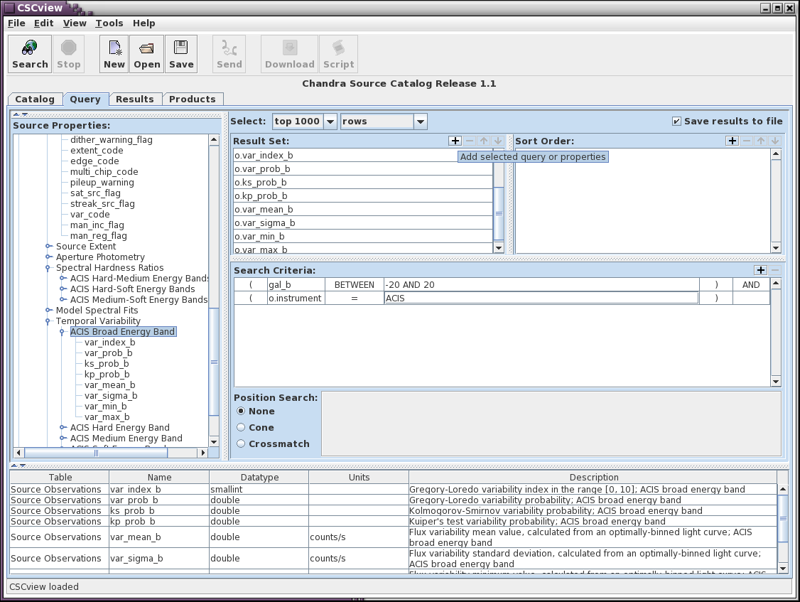
Figure 4: ACIS broad band source observation variability columns added with the '+' button.
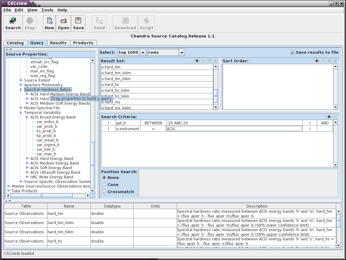
Figure 5: Select the hardness-ratios columns (ie the colors) added by dragging and dropping the group heading into the Result Set
Finish and submit query
The search is almost ready to be submitted. The default form only will return the first 1000 rows. Since the Sort Order was not specified, this will be a random selection. Instead this analysis requires all the available galactic sources be returned as is shown in Figure 6.
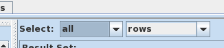
Figure 6: The search needs to return all rows so that a complete sample is available.
Since it is expected that a large number of rows will be returned, the results can be directly saved to a file instead of being presented in the Results tab. For large queries (many columns and/or many rows) this can be more efficient.
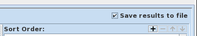
Figure 7 : Save results directly to a file for further analysis
Now the  button can be selected. Since the
results are going to be saved directly to a file, a dialog box is
displayed with path, filename, and format. See Figure 8.
The analysis will be done in
TOPCAT
so the file needs to be saved
in VOTable TABLEDATA format.
button can be selected. Since the
results are going to be saved directly to a file, a dialog box is
displayed with path, filename, and format. See Figure 8.
The analysis will be done in
TOPCAT
so the file needs to be saved
in VOTable TABLEDATA format.
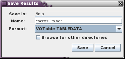
Figure 8: Save results in VOTable format
Selecting Save will then start the query and download. The download dialog box will appear with the Progress message Downloading.... When the Progress changes to Downloaded and the Filesize stops increasing, the query is complete.
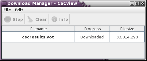
Figure 9: Download progress. When complete, this query generated a 33Mb file.
This query may take several minutes to complete and download based on available bandwidth.
Analysis with TOPCAT
The list of galactic sources with variability and hardness ratios has now been saved in VOTable format, an XML format loosely resembling an HTML table with additional meta-data. This format is increasingly popular for exchanging tabular data within the astronomical community. The TOPCAT catalog tool has native VOTable format support. The CSCView output can be loaded directly from the command line by specifying the -f (format) flag
unix% topcat -f votable /tmp/cscresults.vot
The TOPCAT window is shown in Figure 10 with the CSCView results loaded.
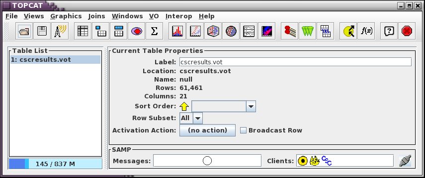
Figure 10: topcat main window. The result returned 61,461 sources (rows)
There were 61,461 rows returned by the query and 21 separate
columns. We can review the columns by selecting the  button and we see the list of columns as in Figure 11.
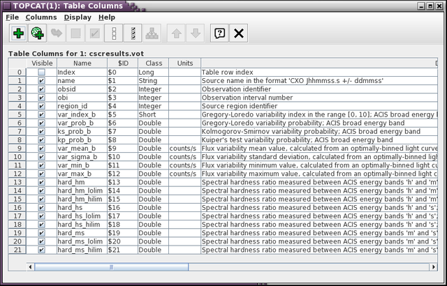
Figure 11: List of columns in the table. The var_prob_b, column number 6, is the Gregory-Loredo variability probability.
The VOTable has not only saved the data, but has save some important meta-data such as column descriptions, units, and data-type.
This analysis will use the ACIS broad band Gregory-Loredo variability probability values, var_prob_b, as the measure of variability. The data needs to be separated into two groups: those sources that are variable, and those that are not considered variable. A probability of 90% is used here as the threshold to classify sources into these two groups.
These groups can be created in TOPCAT using the concept of subsets. A subset
is a non-destructive type of dynamic filter that can be applied to the rows of a table.
Sets are created by selecting the  button in
the main TOPCAT window. The steps to create new steps are shown in Figure 12.
button in
the main TOPCAT window. The steps to create new steps are shown in Figure 12.
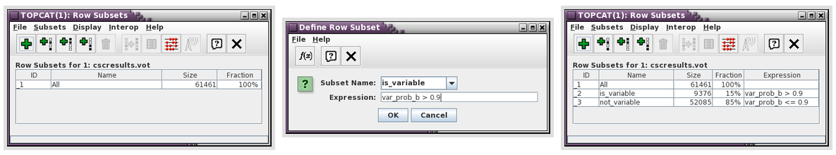
Figure 12: Creating new subset of variable sources
In Figure 12 (Left) is the empty row subsets window. Selecting the add button displays the Define Row Subset dialog box (Center). The first subset that will be created is for the variable sources; it is given the Subset Name is_variable and the expression that defines the subset is typed in the Expression box. This is repeated for the non-variable sources and the final result is shown in the (Right) box where both is_variable and not_variable subsets have been defined. This window also shows that 15% of the sources have been identified as being variable according to the 90% threshold criteria that was selected.
Note: the advantage of using subsets is that they are dynamic. If the subset is changed, for example the variability criteria changed from 90% to 95%, then all the open plots will be updated automatically.
These subsets will now be available in all TOPCAT windows.
One easy way to investigate if there is any relationship between
color and variability is to simply make a histogram of the hardness
ratio values for both groups of sources. This can be done using
TOPCAT's histogram tool,  from
the main window. In Figure 13, the histogram of the hard_hs, hard to soft band hardness
ratio, is selected. From the Row Subsets section the is_variable and not_variable
subsets are selected, and the histograms have been normalized (top button bar, "1" icon fifth from the right).
from
the main window. In Figure 13, the histogram of the hard_hs, hard to soft band hardness
ratio, is selected. From the Row Subsets section the is_variable and not_variable
subsets are selected, and the histograms have been normalized (top button bar, "1" icon fifth from the right).
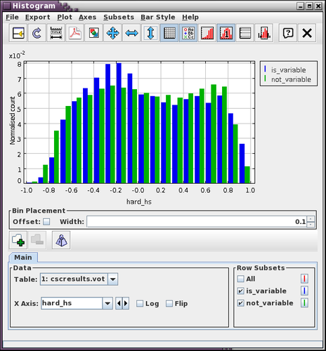
Figure 13: Histogram of hard_hs color for variable and non-variable sources.
Comparing these bi-modal histograms, there are a larger fraction of variable sources with hard_hs in the -0.4 to 0.0 range than non variable source. Since the hardness ratio is defined as hard - soft, values less than zero represent sources with lower energies, suggesting that there may be a class of variable, low energy sources worthy of further analysis.
Possible next steps include returning to CSCView to add the hard_hs constraint into the Search Criteria and returning additional spectral information (spectral fit model parameters, spectrum and response files, etc). A comparison of the other variability measures (Kupiers and Kolmogorov-Smirnov) may also be conducted with the data already retrieved to look for conformation of these results.
Summary
This thread has shown how to use the CSCView GUI to construct and execute a query for properties-based query, rather than focusing on a particular target. It has also shown how to use TOPCAT to categorize and analyze the results to identify specific class of objects that might warrant further study.
Caveats
There are a few caveats about the analysis presented that should be considered when doing such analyzes with the Chandra Source Catalog.
The CSC is biased. Chandra is not a survey mission and only a small fraction of the sky has been observed, and has been observed in configurations optimized differently for each observer's science objectives. However, the fields observed are by virtue of the peer review process the most scientifically interesting currently known.
Chandra observations not typically focused on timing observations unless the spatial resolution is required (eg decay of GRB). So while this thread focused on time variability, most of the objects are likely to have been observed serendipitously.
Finally, the hardness ratio values are based on the observed count rates. This means that the absorption through the galactic plane has not been taken into account. This may further bias the results.
History
| 16 Sep 2013 | Initial version. |