Gallery: Binning
Examples
- Bin Event File to Image; Specify Bin Size
- Bin Event File to Image; Specify Number of Bins
- Bin Event File to Image With Filtering
- Bin Event File to Image With FOV Filtering
- Weighted Binning
- Adaptive Binning
- Adaptive Binning (Polar Coordinates)
- Contour Map Based Binning
- Map Based Binning: Hardness Ratio Map
- Binning Arbitrary Axes
- Alternative binning: hexagonal grid
- Alternative binning: Voronoi tessellation
- Alternative binning: centroid map
- Alternative binning: steepest ascent with pathfinder
- Alternative binning: stack of regions with mkregmap
1) Bin Event File to Image; Specify Bin Size
One of the first things Chandra users want to do is to bin their event file into an image. The ds9 application does this automatically when you load the event file; but when you need to run tools such as wavdetect or csmooth you will need to bin the event file into an image yourself using dmcopy.
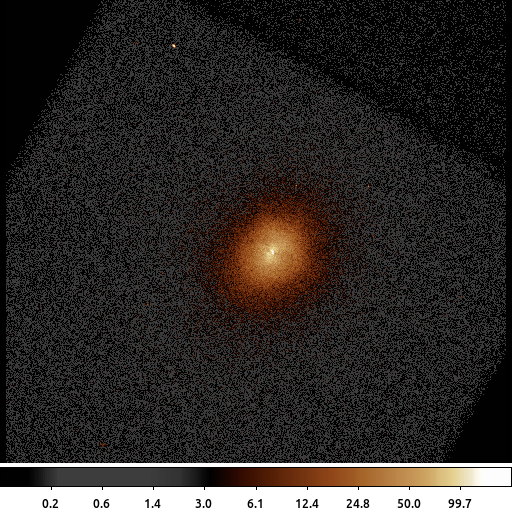
dmcopy "acisf06934N002_evt2.fits[bin x=3500:4500:2,y=3500:4500:2]" 6934_sky_binsize.fits clob+
The following commands can be used to visualize the output
ds9 6934_sky_binsize.fits -scale log -zoom 1 -cmap load $ASCDS_CONTRIB/data/heart.lut
2) Bin Event File to Image; Specify Number of Bins
Rather than specify bin size you can specify number of bins.
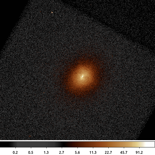
dmcopy "acisf06934N002_evt2.fits[bin x=3500:4500:#512,y=3500:4500:#512]" 6934_sky_nbins.fits clob+
The following commands can be used to visualize the output
ds9 6934_sky_nbins.fits -scale log -zoom 1 -cmap load $ASCDS_CONTRIB/data/heart.lut
This example produces the same output as the example above, but rather than specifying the bin size we specify the number of bins.
3) Bin Event File to Image With Filtering
Typically, users will also need to apply various filters to their datasets when they are binning. In this example we apply a circular spatial filter to the event file as the data are being binned.
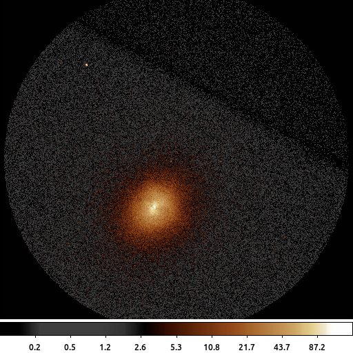
dmcopy "acisf06934N002_evt2.fits[sky=circle(4096.5,4096.5,500)][bin sky=2]" 6934_sky_circle.fits clob+
The following commands can be used to visualize the output
ds9 6934_sky_circle.fits -scale log -zoom 1 -cmap load $ASCDS_CONTRIB/data/heart.lut
In this example, the individual columns X and Y ranges have been replaced with the simplified syntax [bin sky=2]. sky is the name of the vector column, composed of the X and Y columns.
By default the image shrinks to a bounding-box around the filter. Values outside the region are set to 0. This behavior can be changed using DM options.
4) Bin Event File to Image With FOV Filtering
Another common spatial filter is to apply the Field of View file (FOV) to establish the edges of data within the image. The FOV file is a FITS REGION format file that contains at least 1 row per CCD.
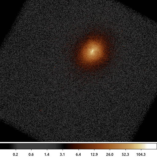
The following commands can be used to visualize the output
ds9 6934_s3.fits -scale log -zoom 1 -cmap load $ASCDS_CONTRIB/data/heart.lut
5) Weighted Binning
We do not always bin to accumulate counts. We can use weighted binning to accumulate other things like flux.

The following commands can be used to visualize the output
ds9 6934_flux.fits -scale log -zoom 1 -cmap load $ASCDS_CONTRIB/data/heart.lut
6) Adaptive Binning
Usually we work with images that are binned such that all the pixels are the same size (and most often, are square). There are applications where having the data binned on an irregular or adaptive grid can be useful. There are many approaches to compute such a grid, in this example we introduce the CIAO tool dmnautilus.
dmnautilus uses a quad-tree algorithm. It works by taking the image and dividing it into 4 approximately equal sub-images. It computes the signal-to-noise (SNR) for each of the sub-images. If the SNR is above the desired threshold, then it further subdivides that sub-image in four. If the SNR is below the threshold, then the process stops for that sub-image tree. The result is a grid where each cell ("pixel") will have at most a SNR equal to the input threshold.
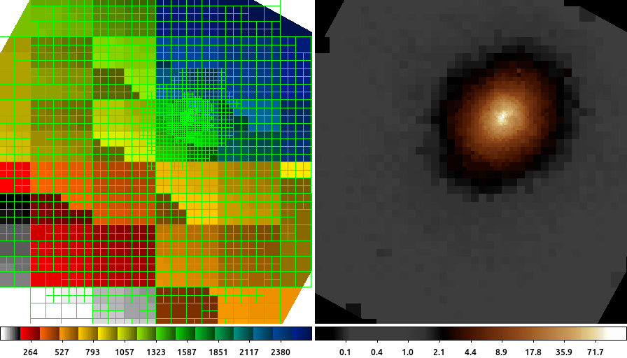
dmnautilus 6934_s3.fits 6934_abin.fits snr=20 outmask=6934_mask.fits clob+
The following commands can be used to visualize the output
ds9 6934_mask.fits 6934_abin.fits  -frame 1 -zoom 1 -cmap load $ASCDS_CONTRIB/data/16_ramps.lut -frame 2 -scale log -cmap load \
    $ASCDS_CONTRIB/data/heart.lut
The image on the Left shows the grid that dmnautilus computed, the 6934_mask.fits output file. Each of the cells in the grid has an upper limit SNR=20 (400 counts) -- single pixel cells that could not be subdivided further can exceed this limit.
The image on the Right shows the data with that binning applied. The boundary of the cluster emission is more easily identified.
7) Adaptive Binning (Polar Coordinates)
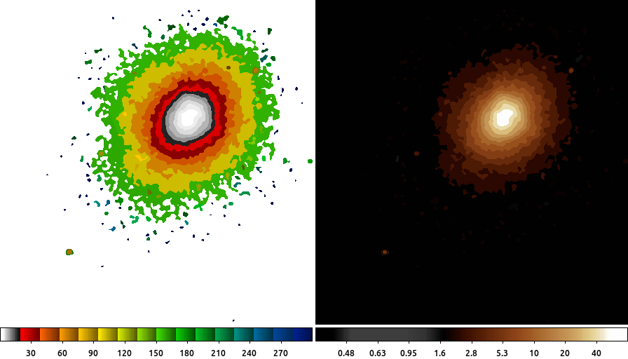
dmradar is the polar equivalent of dmnautilus. Rather than subdivide the image in X and Y, dmradar divides the image in Radius and Angle. This can provide a more natural binning for circular or elliptically shaped emission.

dmradar 6934_s3.fits 6934_rbin.fits snr=20 xcenter=4033.7 ycenter=3956.8 method=0 shape=pie rinner=5 router=500 outmaskfile=6934_rmask.fits clob+
The following commands can be used to visualize the output
ds9 6934_rmask.fits 6934_rbin.fits  -frame 1 -zoom 1 -cmap load $ASCDS_CONTRIB/data/16_ramps.lut -frame 2 -scale log -cmap load \
    $ASCDS_CONTRIB/data/heart.lut
The image on the Left shows the grid that dmradar computed, the 6934_rmask.fits output file. Each of the pie wedged in the grid has an upper limit SNR=20 (400 counts).
The image on the Right shows the data with that binning applied. The boundary of the cluster emission is more easily identified.
8) Contour Map Based Binning
The dmnautilus example above shows one example of an irregular, adaptive binning algorithm. There are several other commonly used adaptive binning algorithms in the community: Weighted Voronoi Tessellation and Contour Binning are probably the most common two.
In this example we introduce the dmmaskbin tool that takes as input a traditional counts (or flux) image along with a pixel-map image (which pixels belong to which group) and uses those to create the binned image.
dmmaskbin 6934_s3.fits 6934_s3.contour.map 6934_cbin.fits clob+
The following commands can be used to visualize the output
ds9 6934_s3.contour.map 6934_cbin.fits -frame 1 -scale linear -cmap load $ASCDS_CONTRIB/data/16_ramps.lut -frame 2 -scale log -cmap load \
    $ASCDS_CONTRIB/data/heart.lut
In this example we have a input map (Left), 6934_s3.contour.map . The pixel value indicates to which group the pixel location belongs.
Right: The output image, 6934_cbin.fits with a contour mapping binning applied. The sum of the pixel values in each group from the input counts image have been normalized by the size of the group and that average value replicated in each pixel in the group in the output image.
9) Map Based Binning: Hardness Ratio Map
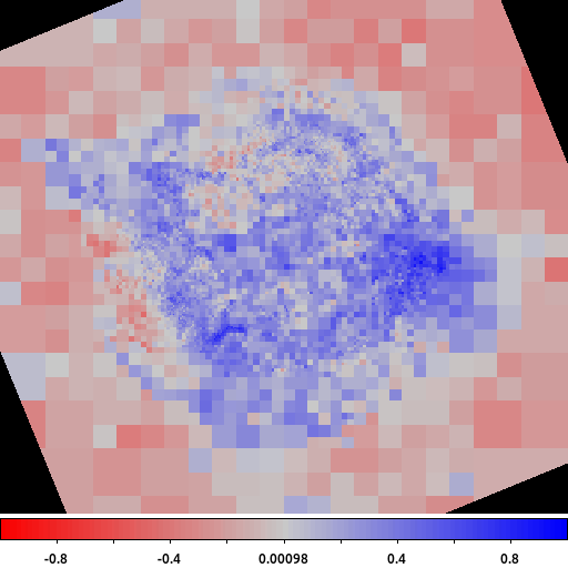
Based on the above two examples we can now create a more useful example: Creating a map of the hardness ratio. For simplicity we define the hardness ratio, R, as
\[ \mathcal{R} = \frac{H-S}{H+S} \]Where H is the number of counts in the hard (high) energy band and S is the number of counts in the soft (low) energy band. So a hardness ratio approaching 1.0 is a region dominated by hard X-ray emission, and values approaching -1.0 are dominated by soft emission.
dmcopy "acisf00214N003_evt2.fits[sky=region(acisf00214_000N003_fov1.fits[ccd_id=7]),energy=500:7000]" cas_a.fits clob+
dmnautilus "cas_a.fits[bin sky=2]" cas_a_bin.fits snr=20 outmask=cas_a_broad.map clob+
dmmaskbin "cas_a.fits[energy=500:1500][bin sky=2]" cas_a_broad.map soft.fits  clob+
dmmaskbin "cas_a.fits[energy=1500:7000][bin sky=2]" cas_a_broad.map hard.fits  clob+
dmimgcalc soft.fits,hard.fits none hardness.map op="imgout=((img2-img1)/(img2+img1))" clob+
The following commands can be used to visualize the output
ds9 hardness.map -zoom 1 -cmap load $ASCDS_CONTRIB/data/004-phase.lut -cmap invert yes -scale limits -1 1 -view colorbar yes
In this example we take the event file for CasA and apply the spatial binning and energy filtering we saw in the earlier examples.
We then run dmnautilus on the broad band, ie combine hard+soft bands, to create a grid where we have a combined SNR limit of 20 (ie a limit of 400 counts).
We then use this map to create an image of the soft band and hard band counts.
And the finally we combine those two images using the equation above to compute the hardness ratio map.
Since we have selected the bins to include roughly 400 counts each, the statistical error in this map is low.
We can clearly see from this map the hard emission in the Western part of the remnant. (North is towards the top of the image).
10) Binning Arbitrary Axes
So far all the binning example have been of data in sky coordinates. However, we can bin data on any column in the input table.
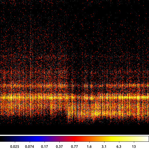
In this example we will show a quick way to generate thousands of spectra using the data from the hardness ratio example.
The following commands can be used to visualize the output
ds9 cas_a.spectra.img -pan to 2200 230 physical -scale log -cmap b
This thread starts by using dmimgpick to add a new column to the event file. The new column is called cas_a_broad_map. The tool looks up the sky position for each event and then uses the closest value in the map file to populate the new column.
Next we use dmcopy to create an image but not in sky coordinates. In this example the X-axis is the value of the cas_a_broad_map column; ie the group ID. The Y-axis is binned on pi, which is the observed energy channel.
The results: We now have an image where each column is the spectrum for different parts of the sky. The image above shows just a small segment of the total image zoomed into a region where we can clearly see the change in the spectral signature.
Note: This type of spectrum is not immediately useful with CIAO, as we do not have the appropriate response files (ARF and RMF), nor do we have the information we need to account for background (including area scaling information).
11) Alternative binning: hexagonal grid
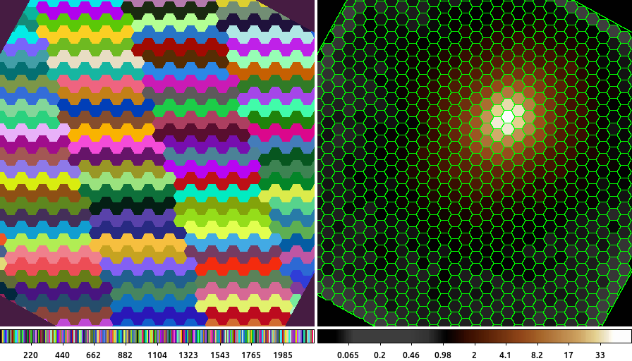
Typically we bin images into square (or more rarely rectangular) pixels which approximates the physical geometry of the detector elements (ie physical pixels on a CCD). The hexgrid tool allows users to create a hexagonal grid to bin the data. Why hexagonal? It turns out that a hexagon is the highest order regular polygon (equal length sides) that can be used to uniformly tile a 2D plane. As such, it's the closest approximation to a circle; and since the PSF is generally circular (or at least elliptical), it may be a closer match to observed sources.
The hexgrid tool creates a grid of hexagons, with equal side lengths. The output map file is an image whose pixel values identify with hexagonal group each (square) pixel belongs to.
The following commands can be used to visualize the output
ds9 hex.map 6934_s3.hex10.fits  -frame 1 -zoom 1 -linear -cmap load $ASCDS_CONTRIB/data/005-random.lut -frame 2 -scale log -cmap load \
    $ASCDS_CONTRIB/data/heart.lut -region hex.reg
In this example we created a hexagonal grid where each hexagon is has a side length equal to 10 pixels. The input image was filtered with the field-of-view file so that the tool knows where the edge of the detector is and leaves those pixels ungrouped (map value equal to 0). The map file is shown in the left-hand side of the image. For the color map we have chosen a random set of colors to help highlight the different map ID values.
The output map output is then run through the map2reg script to create a region file from the map grid; one region is created for each map ID value found in the input map file. Note: since the map ID values are not necessarily continous nor do they necessarily start at 1, the row number (not component value) in the region file may not correspond to the map ID value in the input file. This file can be used to easily display the map grid as is shown in the right-hand side image.
As is shown in other Gallery examples, the dmmaskbin tool is then used to apply the map file (unfortunately the terms "mask" and "map" are sometimes used interchangeably) to the original counts image which is what is display in the right-hand side image.
12) Alternative binning: Voronoi tessellation
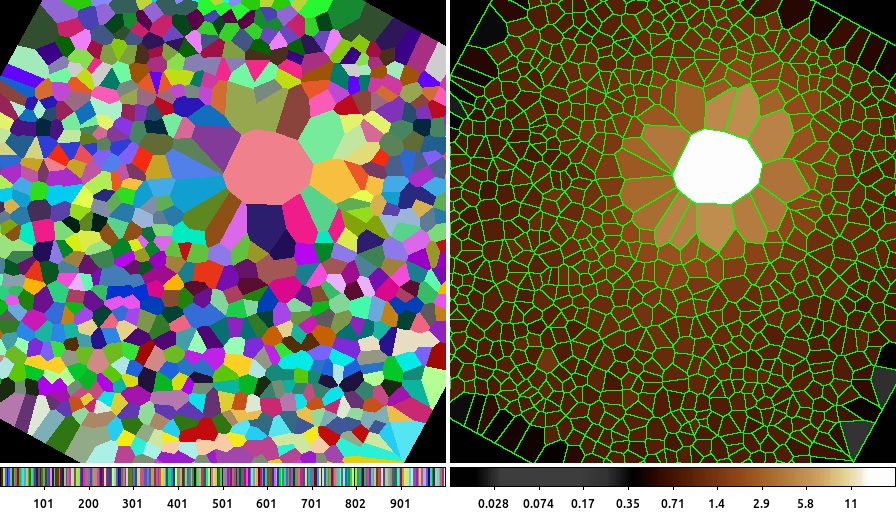
Another alternative binning technique is to create a grid based on a Voronoi Tessellation of points. The key feature of the Voronoi tessellation is that each cell is a convex hull that encloses each point. By default, the vtbin tool selects the set of points that represents the local maxia in the image. Since we are working with low count data, we want to avoid many spurious "1 count" kind of local maxima caused by random fluctuation so this technique works best when the image is smoothed.
The following commands can be used to visualize the output
ds9 vt.map 6934_s3.vt.fits  -frame 1 -zoom 1 -linear -cmap load $ASCDS_CONTRIB/data/005-random.lut -frame 2 -scale log -cmap load \
    $ASCDS_CONTRIB/data/heart.lut -region vt.reg
In the left hand frame we see the map created by vtbin. As with the hexgrid example, the pixel values represent the map ID for each region; the color map is a set of random colors to show the different regions. The right hand frame shows the output image after the map file has been applied to the original input image using the dmmaskbin tool with the region file created by map2reg overlaid.
The choice of the initial central points is the key to this algorithm. The default is to use the local maxima however users can supply their own set of points which is used by the centroid_map script.
13) Alternative binning: centroid map
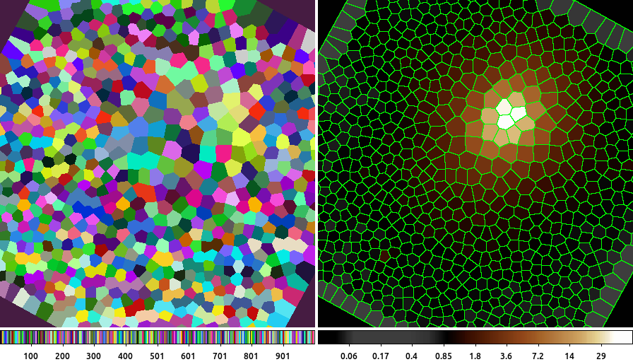
The vtbin output can contain highly irregular shapes, though adhering to the condition that each is a convex polygon. The centroid_map script takes this a step further. It runs vtbin to generate an initial set of polygon regions. It then computes the centroid of the events in each polygon and then uses those centroids as input to vtbin to compute a new set of polygon regions. This process is repeated a specified number of time. [Theoretically this algorithm would converge so that the centroids would not shift between iterations, but it does so somewhat slowly especially at the edges of the data.]
The end result is that the output map file generally has much more uniform, generally hexagonal shapes.
aconvolve 6934_s3.fits 6934_s3_sm.fits "lib:gaus(2,5,1,3,3)" method=slide edge=const const=0 clob+
centroid_map 6934_s3_sm.fits"[sky=region(s3.fov)][opt full]" centroid.map numiter=10 clob+
map2reg centroid.map centroid.reg clob+
dmmaskbin 6934_s3.fits centroid.map"[opt type=i4]" 6934_s3.centroid.fits clob+
The following commands can be used to visualize the output
ds9 centroid.map 6934_s3.centroid.fits  -frame 1 -zoom 1 -linear -cmap load $ASCDS_CONTRIB/data/005-random.lut -frame 2 -scale log -cmap load \
    $ASCDS_CONTRIB/data/heart.lut -region centroid.reg
This is similar to the vtbin example showing the map file on the left and the binned image on the right. The polygons are now more uniform in size and spacing. For very bright sources, the polgyons can become very small; users can use the scale parameter to select different pixel scaling when computing the centroid which will lessen the impact of bright pixels.
14) Alternative binning: steepest ascent with pathfinder
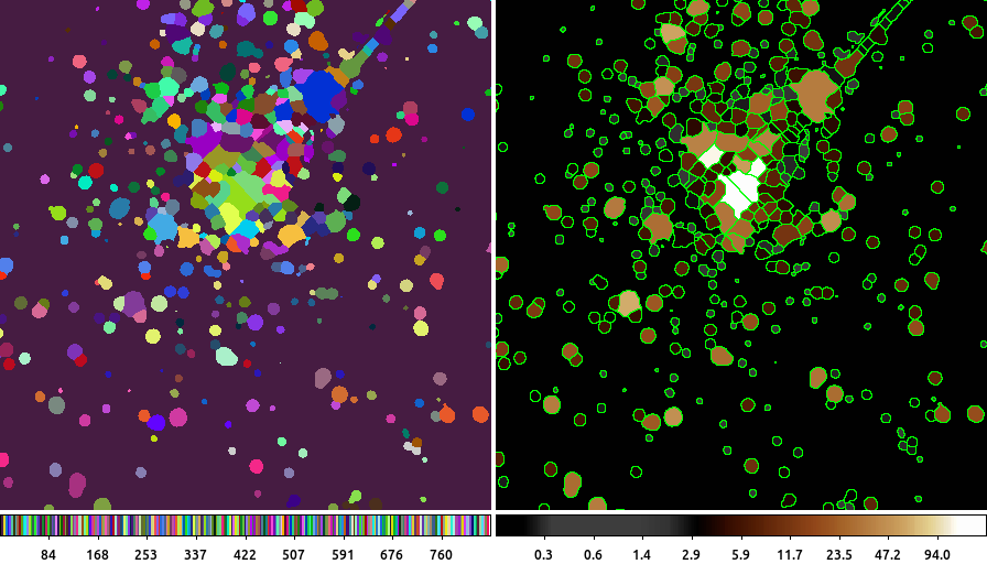
The dmimgblob tool creates a map file by identifying clusters of connected pixels that share a side and assigning each separate cluster to a separate group. The pathfinder tool is somewhat similar but instead of grouping all pixels together it creates groups by following the steepest gradient from one pixel to its neighbors until it finds a local maxima. All pixels whose steepest ascent gradient that reach the same maxima are grouped together. This has the advantage that it can separate nearby point sources. This tool is better suited for grouping images with many point (or point-like) sources. It also works best when the input image is smoothed so that it can find the steepest gradient without needing to worry about statistical noise.
aconvolve "acisf04396_broad_thresh.img[bin sky=2]" orion.img "lib:gaus(2,5,5,2,2)" clob+
pathfinder orion.img pathfinder.map minval=1.0 clob+
map2reg pathfinder.map pathfinder.reg clob+
dmmaskbin orion.img pathfinder.map"[opt type=i4]" orion.pf.fits clob+
The following commands can be used to visualize the output
ds9 pathfinder.map orion.pf.fits  -frame 1 -zoom 1 -linear -cmap load $ASCDS_CONTRIB/data/005-random.lut -frame 2 -scale log -cmap load \
    $ASCDS_CONTRIB/data/heart.lut -region pathfinder.reg
In this example of the star forming region in Orion, there are many individual point sources and with diffuse emission in the center. The algorithm is able to separate many of the individual stars based on the gradient searching algorithm. The left image shows the map file with a random color map applied. The right image shows the output by binning the original image with the map file.
The amount of smoothing can have significant impact on the algorithm. Using an adaptive smoothing tool like dmimgadapt or csmooth may help to provide even better source separation. Subtracting the background may also help to resolve all the point sources embedded in the extended emission.
15) Alternative binning: stack of regions with mkregmap
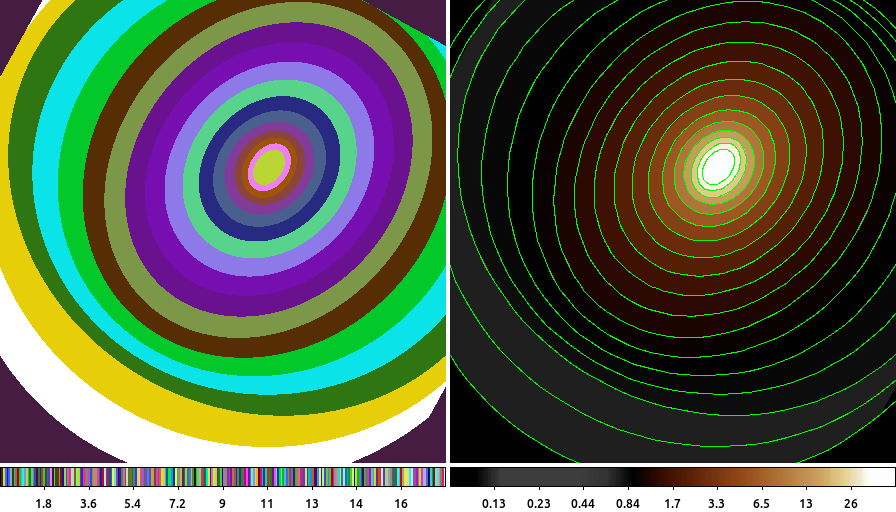
Another way to group data is with a stack of regions; that is use a set of arbitrary regions to define each of the map IDs. The regions can be uniformly created using the pgrid() or rgrid() stack syntax, an arbitray list of regions provided using the @filename syntax, or as shown in this example a set of automatically created contour regions created by the dmellipse tool.
In this example we create a set of elliptical contours that enclose 5%, 10%, 15%, ... up to 95% of the total counts in the image. We then create a map file using the mkregmap script. The stack of regions is specified using the igrid() syntax.
The following commands can be used to visualize the output
ds9 region.map 6934_s3.region.fits  -frame 1 -zoom 1 -linear -cmap load $ASCDS_CONTRIB/data/005-random.lut -frame 2 -scale log -cmap load \
    $ASCDS_CONTRIB/data/heart.lut -region ell.fits
The map file (left image) created from the mkregmap script shown with random colors. The right image shows the map file applied to the original image. Since the region files are actually input to the script there is not need to use map2reg to create them; we can just directly overlay the contours on the binned image.
Question: How did we select the number "18" in the igrid(1:18:1) syntax? Answer:
unix% dmlist ell.fits counts
18