
Less detailed version of this page
Soon after release of the new gain calibration (Jun 2020, CALDB 4.9.2) it was discovered that the LETG/HRC-S background filter was sometimes removing more than the intended 1% of valid X-ray events. A revised calibration was prepared (Jun 2021) and was released in CALDB 4.9.6. See here for details.
The purpose of a gain map is to obtain, for any given X-ray energy, identical pulse height distributions (PHDs) from all areas of the detector at all times. A simple linear scaling of the PHDs does a pretty good job, but as described in section 3.4 of the 2008 gain calibration, a more complicated equation is required to account for energy dependent gain effects, which were seen across all three HRC-S plates in pre-flight laboratory flat field data. That calibration worked well for several years, including right after the March 2012 high voltage change to restore the HRC-S QE and gain, but by around 2015, when detector gain was down to less than half what it was during lab calibration, the adjustments for energy dependence were causing significant distortions to the gain-adjusted PHDs (see bottom panel). Since there is no practical way to recalibrate the energy dependent effects using flight data, this new (2019/2020) calibration reverts to simple linear adjustments, which provide adequately consistent PHD shapes even at very low gains (top panel).
The new calibration benefits from several improvements over the 2008 calibration:
The primary practical result of the gain calibration is that pulse height filtering can be applied to LETG spectra as a function of dispersed wavelength in order to reduce background by over half longward of 20 Å, compared with standard Level 2 processing.
The new t_gmap and pireg_tgmap files resulting from this work will have their version numbers (N000#) incremented by 1.
A key reference is the 2018 Interface Control Document. The AXAF_TGAIN block of the gain map file (hrcsD<date>t_gmapN<version>) contains:
The current (dating from 2008) LETG/HRC-S PI Region Filter (a.k.a. PI/tg_mlam filter) is hrc/tgpimask2/letgD1999-07-22pireg_tgmap_N0001.fits and is also being updated.
Spatial gain (GAINMAP) coefficients are derived from laboratory calibration data and then adjusted to account for gain changes between then and the 2001.5 reference date used for TGAIN calibration. We use the lab calibration results from the 2008 work with a few minor changes:
Gain changes during flight are monitored by measuring pulse height amplitudes over time, using data from frequently observed continuum sources. HZ 43 covers longer wavelengths, mostly on the outer plates. PKS 2155 and Mkn 421 cover shorter wavelengths, mostly on the inner plate. Calibration around the plate gaps has larger uncertainties because emission from all three sources is relatively weak at those wavelengths (roughly 50-70 Å).
As described in
Corrections for Higher Order Diffraction,
PKS 2155 and Mkn 421 spectra have significant contamination
from higher order diffraction, which shifts pulse height
distributions (PHDs) to higher channels than for pure 1st order emission.
These effects can be modeled, but in order to check the accuracy
of our corrections we also analyze data from three bright novae,
RS Oph, KT Eri, and Nova SMC 2016,
that have emission over relatively narrow wavelength ranges
with minimal higher order contamination.
A table of the observations is listed below, along with
plots of spectra.
Table 1
| Source | Wavelengths (Å) | Dates | ObsIDs (old HV, new HV) |
|---|---|---|---|
| HZ 43 | λ ≳ 55 | Nov 1999-Nov 2019 | 59, 1170 (Y=10'), 1011, 1012, 2584, 2585, 3676, 3677, 5042, 5044, 5957, 5959, 6473, 6475, 8274, 10622, 11933, 13025, 14238, 14422, 15465, 16375, 18365, 17323, 19840, 19839, 19971, 20707, 20708, 20706, 21785, 21784 |
| PKS 2155 | λ ≲ 80 | Dec 1999-Jul 2008 | 331, 1704, 1013, 3166, 3709/4406, 5172, 6923, 6922/7295/7294, 8379, 9707/9709/9711 (*/* = same epoch) |
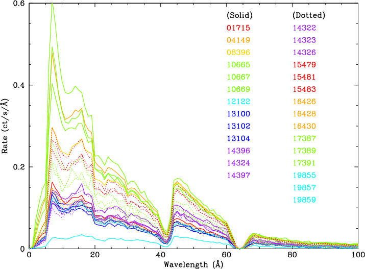
| Mkn 421 | λ ≲ 80 | May 2000-Jul 2019 (only 3 obs before 2010) |
1715, 4149, 8396, 10665/10667/10669, 12122,
13100/13102/13104, 14396/14324/14397, 14322/14323/14326,15479/15481/15483, 16426/16428/16430, 17387/17389/17391, 19855/19857/19859, 19444/20942/20943/20944, 20712/20714/20716, 21818/21820/21822 |
| RS Oph | 14 ≲λ ≲ 35 | Mar-Apr 2006 | 7296, 7297 |
| KT Eri | 20 ≲ λ ≲ 50 | Jan-Apr 2010 | 12097, 12100, 12101, 12203 |
| Nova SMC 2016 | 20 ≲ λ ≲ 53 | Nov 2016, Jan 2017 | 19011, 19012 |
|
|
| |
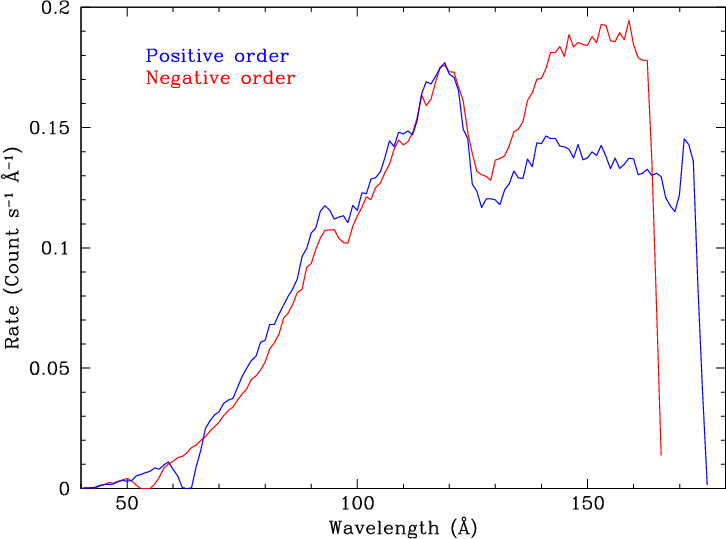
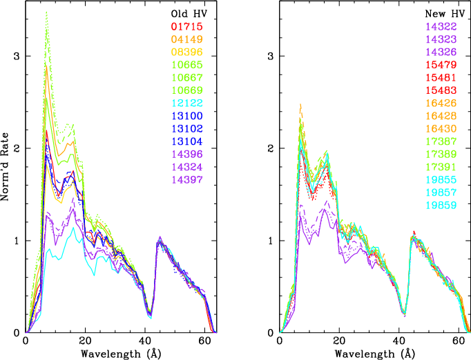
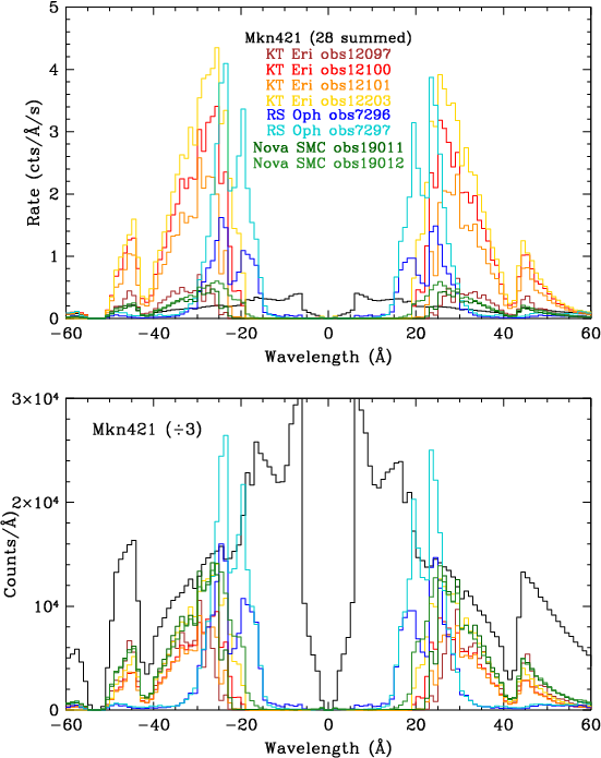
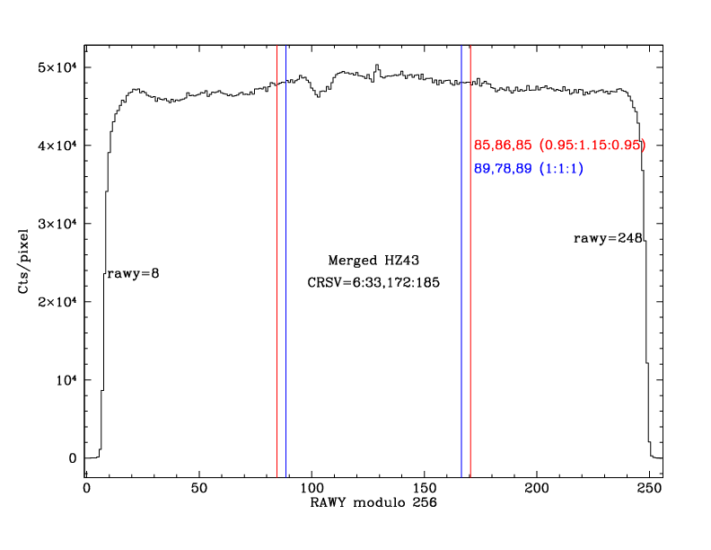
| Fig. 1: [pdf] HZ 43 spectrum. | Fig. 2: [pdf] Mkn 421 spectra (positive order) through June 2017, illustrating rate variations. | Fig. 3: [pdf] Mkn 421 spectra normalized to rates at 45 Å, showing spectral shape variations. |
|
| |||
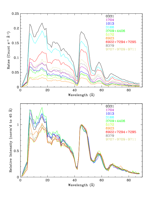
| Fig. 4: [pdf] Top: PKS 2155 spectra (summed + and - orders). Bottom: Rates are normalized to those at 45 Å, as in Fig. 3, to illustrate variations in spectral hardness, and therefore higher order contamination. | Fig. 5: [pdf] Spectra of Mkn 421 (summed though 2017), RS Oph, KT Eri, and Nova SMC 2016. Spectra of the last three sources are largely free of higher orders, unlike PKS 2155 and Mkn 421. Observations of RS Oph and KT Eri had saturated telemetry (partial for ObsID 12097) so true rates are higher than indicated. Binning is 1 Å to smooth out sharp features. |
All data are reprocessed from Level 1 to Level 2 using the updated (May 2017, CALDB 4.7.4) HRC-S BADPIX and QEU files, along with some extra steps:
All periods of elevated detector background are removed (more stringently than in the 2008 analysis) and then the data are dewiggled, detilted, and symmetrized following steps described here, and spectra are extracted using the S/N-optimized region described on the bottom of that page, with background regions of the same size and shape offset by 85 pixels on either side (BACKSCAL=2). To characterize the detector gain at a given time and detector location we compute the median of SAMP from the background-subtracted PHDs, and uncertainties are estimated as the variance (excluding the 0-5 and 95-100 percentiles) divided by the square root of the number of counts in the truncated range.
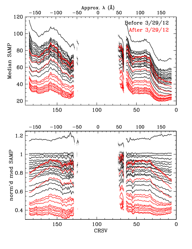
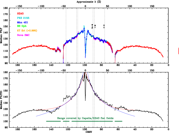
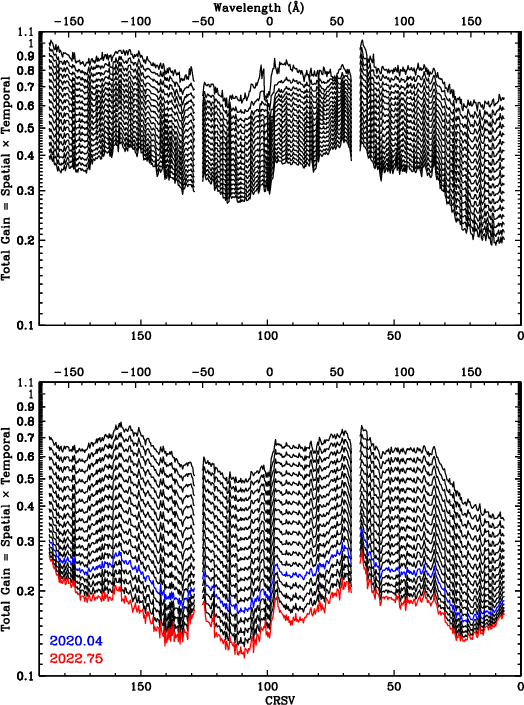
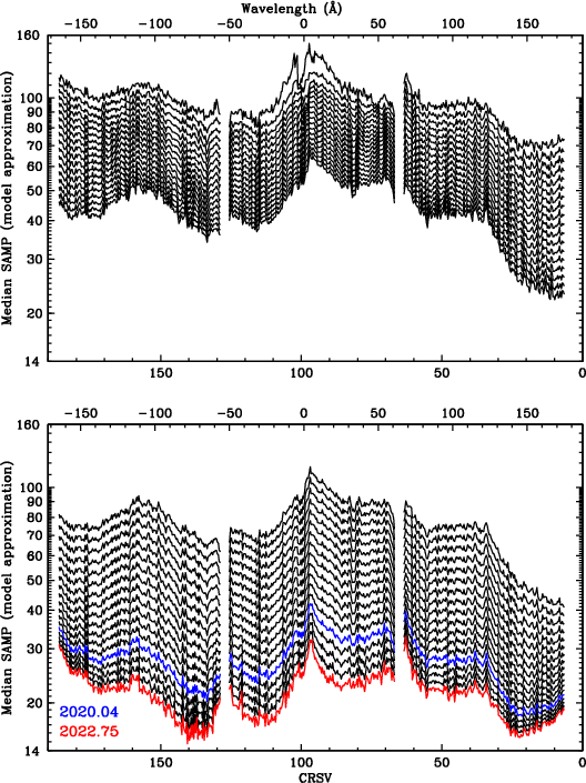
Figure 6 plots median SAMP as f(CRSV) for all HZ 43 observations. As seen in the top panel, gain varies a great deal across the HRC-S. To better illustrate time-dependent trends, the bottom panel normalizes median SAMP to the values found from ObsIDs 1011 and 1012. It is interesting to note that gain dropped more quickly on the outer half of the outer plates prior to the HV change in late March 2012, that gain did not recover as completely there after the change, and that the rate of gain loss there has since been lower than in the inner half of the plates.
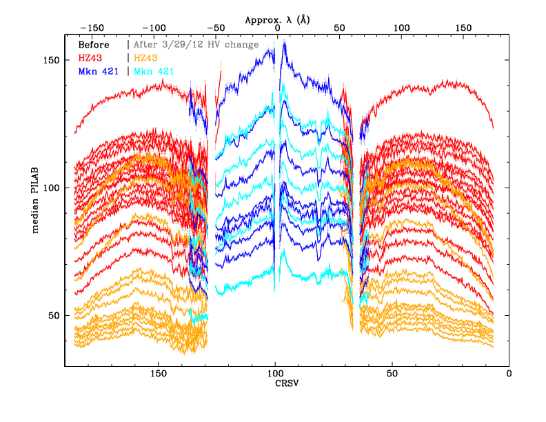
The new GAINMAP is then applied to all the flight analysis data to calculate PILAB (PI using LAB spatial gain map) from SAMP. Median PILAB values are then measured for background-subtracted spectra for each CRSV subtap, with results shown in Figure 7. The advantage of using PILAB instead of SAMP is that the effects of local spatial gain variations are largely removed. This is particularly important when background contamination of the spectrum is relatively high, as the background data come from regions that are offset from the spectral region; minimizing variations in PHD shapes as a function of CRSU minimizes systematic biases that might arise during subtraction of the background PHDs.
Applying spatial gain corrections before calibrating time-dependent changes also minimizes systematic biases that might arise from differences in spatial sampling of detector gains from one observation to another (even when background is negligible) as the aim point drifts over time. As an example, early in the mission, CRSU subtap 9a was sometimes included in extracted spectra but over the years as the aim point drifted toward small CRSU, the edge of the spectrum moved to 8c and then 8b. Similar arguments apply to the drift in CRSV, which can also lead to wavelength-dependent effects near abrupt changes in the CsI photocathode's electron yield and thus the effective gain.
|
| |
| Fig. 6: [pdf] Median SAMP vs CRSV with 1-tap bins (HZ 43 data through Nov 2019), showing only points with error<2.0%. Bottom panel shows values normalized to the average of ObsIDs 1011 and 1012, corresponding to around 2001.5, when gain was roughly the same as during pre-flight laboratory calibration. | Fig. 7: [pdf] Median PILAB vs CRSV with 1/3-tap bins. PILAB is SAMP with the lab spatial gain (GAINMAP) corrections; no higher-order-diffraction or time-dependent (TGAIN) corrections have been applied. With spatial gain variations largely (but not fully) removed, the general shape of the curves is determined mostly by the detector energy response, tending toward higher pulse heights as energy increases. The dips around the plate gaps (CRSV~130 and 60) and outer edges are caused by higher than average gain losses that occured between lab calibration and early in the mission (see Flight-Based Adjustments to Spatial Gain Map section). (Observations through July 2019.) |
As seen in Figures 6 and 7, gain varies over time, and in order to apply time-independent pulse-height filters on the data we must calibrate the time dependence, which we do for each subtap.
As noted above, higher orders (HOs) contribute significantly to the spectra of Mkn 421 and PKS 2155 at all but the shortest wavelengths. Those HOs create higher-channel PHDs in the HRC-S, and our analysis must account for these effects. HZ43 also has some 2nd order contamination beyond mλ~90 Å, and 3rd order beyond ~130 Å, but this can be completely ignored because the HO contributions are generally <1% and PHD medians are essentially constant longward of ~70 Å. The novae (RS Oph, KT Eri, and Nova SMC 2016) have essentially pure 1st order spectra out to at least 30 Å (even beyond the C-K edge for some ObsIDs), and nearly pure higher-order spectra at longer wavelengths. They are also bright enough to be good test cases for the accuracy of our corrections for HOs at large mλ by comparing their corrected median PI values with results from HZ43.
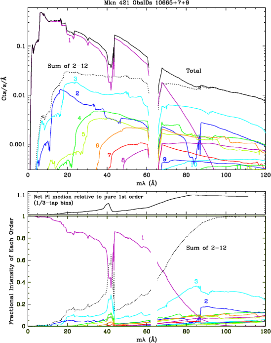
The first step is to create gARFs (effective area curves) for plus and minus orders 1-12 of each spectrum, and then fit spectra using Sherpa to determine each order's flux as f(λ). Mkn 421 and PKS 2155 are fitted using absorbed broken power-law models (see Fig. 8 example). The very complicated spectra of the novae (RS Oph, KT Eri, and Nova SMC 2016) are impractical to fit so we use a program that iteratively subtracts higher orders to yield a pure 1st order, which is then used to compute the HO fluxes by the ratios of their gARFs.
The measured median PI value is then modeled as the flux-weighted average of each order's median PI, using the PI vs λ relationship derived from the 2008 calibration and shown in Figure 9 (which is very similar to the result of the present calibration, shown in Figure 28). Effective fluxes within each tap (as opposed to within a wavelength interval) are computed by summing over the full wavelength range of a given tap (covering 151 0.0125-Å bins) after convolving each bin with the double-cusp dither pattern (about 186 bins). The slightly different wavelength coverage of a given tap from one observation to another, caused by aim point drift, is also accounted for by standardizing to 0th order centered on the "permanent" aim point of CHIPY=8915 (corresponding to degapped RAWY=25375, or CRSV=99.121); the effect on median PI is only appreciable (~1%) at the shortest wavelengths. Correction uncertainties are estimated as 1/5 of the correction magnitude, and net error is computed by adding that error in quadrature with the original statistical error from measuring the median pulse height. The magnitude of HO corrections for one of the harder Mkn 421 spectra is shown in the short middle panel of Figure 8. Figure 10 compares before- and after-correction median PILAB values for a sample of subtaps (one out of every nine) on each plate.
See here for more details on how HO contamination
and its effect on PHD medians were measured.
|

|
| Fig. 8: [pdf] Top: Fits to 12 +orders of Mkn 421 combined ObsIDs 10665,10667,10669. Middle: Ratio of measured median PI to 1st order median PI without any higher-order contamination. Bottom: Relative contributions of each order. | Fig. 9: [pdf] Median PI vs λ relationship (+ and - orders) based on incomplete 2017 analysis results, used to model the effects of higher order contamination. The discontinuity near 20 Å is from the I-M edge, which appears to cause a small but real jump in the PHD median, presumably from a change in the photocathode electron yield. (Comparison with the corresponding plot from the 2008 calibration [pdf] illustrates the improved agreement between sources, and between + and - orders, particularly near the plate gaps (around 50-70 Å). Self-consistency of results from the current (2020) analysis is even more impressive. |
|
|
|

| |
|
Corrected: [pdf] Uncorrected: [png] [pdf] |
Corrected: [pdf] Uncorrected: [png] [pdf] |
Corrected: [pdf] Uncorrected: [png] [pdf] |
Fig. 11: Fits to HO-corrected data (only 1st page shown). [87-page pdf]. 98abc, 99abc, 100a will be interpolated. | |
|
Fig. 10:
Median PILAB vs. time for selected subtaps after correction for higher orders (with error/median < 3%). HZ43 points are effectively free of higher order contamination. Corresponding plots without HO corrections are also listed. | ||||
Time-dependent gain is determined from fits to the data from each subtap (Fig. 11). The model used for the old HV setting is an exponential plus 3rd order polynomial, and an exponential plus constant for the new HV setting. Parameters for taps 98 and 99 and the first third of tap 100, around the aim point where there are few or no usable dispersed spectra, are interpolated from subtaps 97c and 100b.
Median PILAB values are computed from the fits at 18 epochs, one set for each HV setting. The old-HV epochs are chosen to characterize the gain at approximately equal fractional gain-loss intervals, ranging from 135 to 436 days. The first epoch marks the first HRC-S observation (ObsID 1299) on Sep 4 1999 and the 18th is the date of the last observation using the old HV setting, ObsID 14397, on Jul 4 2012. At the earliest times, when gain loss was most rapid and there were only one or two calibration observations, fits are not well constrained, so the first-epoch curve in Figure 12 has relatively large uncertainties. New-HV epochs are separated by 200 to 250 days, beginning with ObsID 14238 on Mar 18 2012--the 1-ks test observation on Jan 9 2012 is ignored--with the last on Oct 2 2022. Observations beyond the last date would be processed using extrapolated gains, but a new calibration and/or HV setting (the latter requiring a third TGAIN file) should be in place before then. Lastly, median PILAB values are normalized to model values at the middle of 2001, when gains are approximately the same as during the pre-flight calibration.
Those relative gain values are used as TGAIN coefficients (see Gain Map Structure above) to compute PI values according to PI(t)=PILAB/C(t) where C(t) is the 1D (dispersion-axis only) TGAIN coefficient. As noted in the Introduction, the new gain calibration uses a slightly different and simpler form of equation than before (see Equation 1 in the Interface Control Document), specifically
PI(t)=((a1/mij)[SAMP/Sij - bij] +a0)/Ci(t)
with the further simplification that bij and a0 are set to zero and mij=1 so that the equation resolves to
PI(t)=a1(SAMP/Sij)/Ci(t)
where Sij is a 2D scaling factor derived from the lab calibration and a1 is a convenient global scaling factor. This is implemented in the GAINMAP section of the AXAF_TGAIN block of the CALDB t_gmap file using two 2D coefficients, with Gij0=0 (kept for backwards compatibility and to minimize software changes) and Gij1=a1/Sij.

|
| Fig. 12: [pdf] Gains for the 18 CALDB epochs (top panel for old HV, bottom for new), normalized to the gain in 2001.5. Both panels' vertical axes cover a factor of 5.5 in gain change; about 13 years are covered in the top panel and 10.5 in the bottom. The green curve in the top panel is for 2001.22, when gains are close to those during lab calibration, and the blue curve in the bottom panel is the gain around the time of this time-dependence calibration (Jan 2020). Bottommost curve is for Oct 2 2022. |
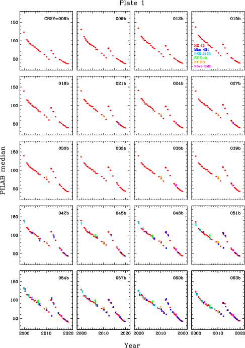
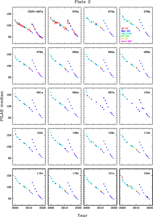
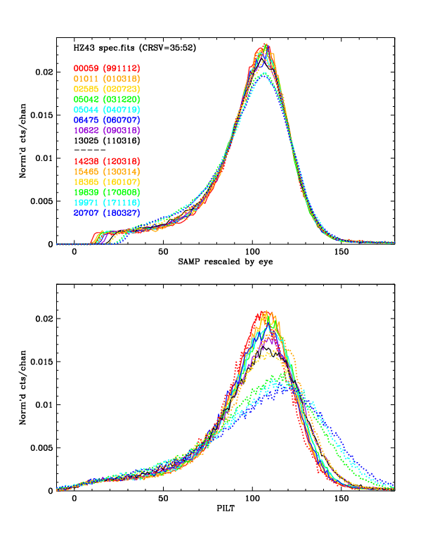
With the TGAIN calibration complete, we can apply time dependence corrections to create the PILT (PI with Lab and Time corrections) column, merge all the on-axis LETG/HRC-S observations of a given source, and extract and analyze PILT PHDs to provide much higher statistical precision than with individual observations.
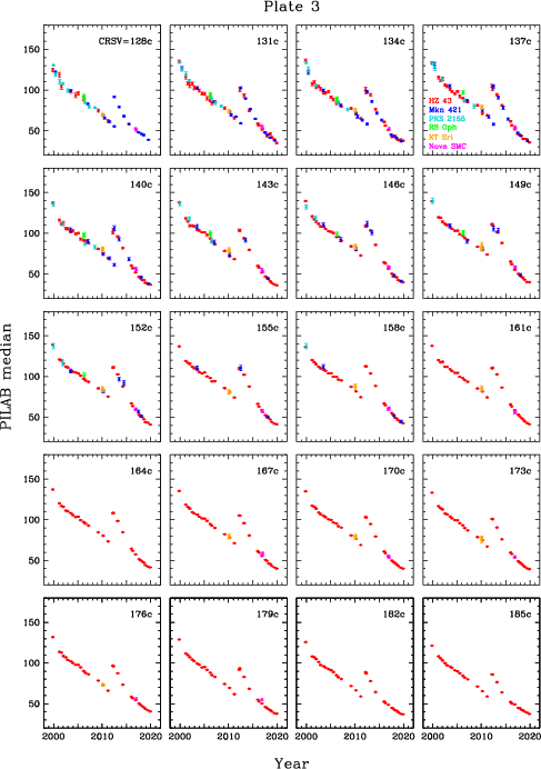
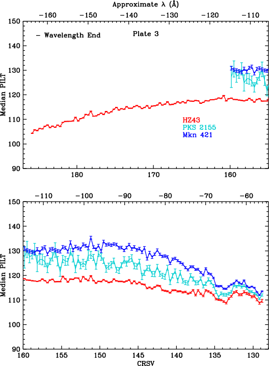
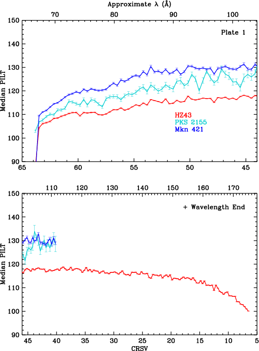
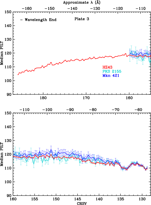
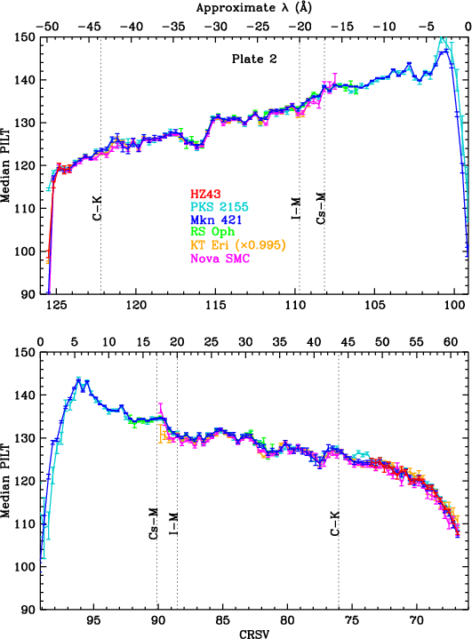
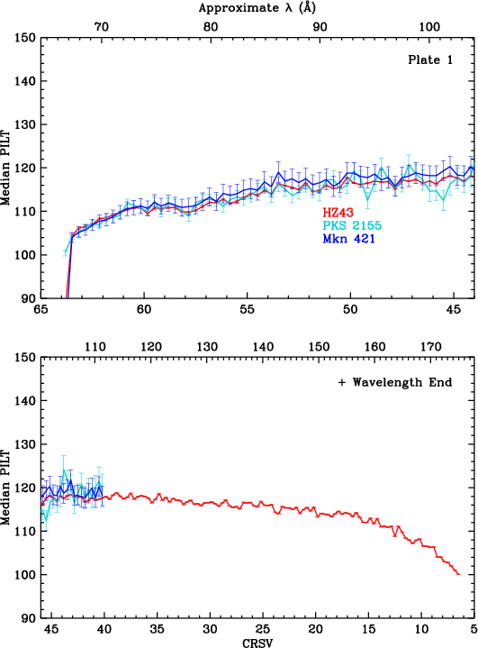
Results are shown for each plate in Fig. 13, before applying corrections for higher order contamination. HO corrections for the merged data were calculated for each CRSV subtap by averaging the count-weighted corrections for each ObsID, yielding the results in Fig. 14. As can be seen, PILT medians are reassuringly consistent for all sources, illustrating that the HO corrections are quite accurate, even for Mkn 421 and PKS 2155 at very long wavelengths where their spectra are entirely from higher orders, and around the C-K edge, where the nova spectra (from RS Oph, KT Eri, and Nova SMC 2016) have little or no HO contamination. (Uncertainties on HO corrections are conservatively set at 20% in the figures.)
|

|
|
| Fig. 13: [pdf3, pdf2, pdf1] Median PILT versus CRSV subtap, using merged data, before applying Higher Order corrections. | ||
|
|
|
| Fig. 14: [pdf3, pdf2, pdf1] Same as Fig. 13, but with HO corrections. Gain changes that occurred between preflight lab calibration and the 2001.5 reference date are most pronounced near the plate gaps and aim point. Cs-M and I-M absorption edges (17.06/16.74 and 20.02/19.65 Å, respectively) are marked because they may cause small jumps in the photocathode electron yield and therefore in the median; elsewhere the curves should vary smoothly. | ||
At this point in the analysis we have a good calibration of the time dependence for each subtap's gain while in orbit (all relative to the 2001.5 reference date), and of relative gain variations on subtap scales, but nothing tying the flight gain directly to gains calibrated in the laboratory. Median PILT should vary smoothly with wavelength, perhaps with some features near absorption edges in the photocathode, but as seen in Fig. 14 there is obvious residual gain variation at small scales all along the detector, large gain drops near the aim point (0th order) and the plate gaps, and probable gain droop at the ends of the outer plates. These deviations are the result of gain changes that occurred between lab calibration and early in the mission.
(This and other sections on the flat field HZ43 observations are included to document the work done. In the end, however, these observations were found to be less useful for gain calibration than expected, and other data and analysis methods provided more reliable results over the detector areas in question.)
Gain calibration near the plate gaps (roughly ±60 Å) is more difficult than elsewhere because our primary calibration sources are all fairly weak at those wavelengths, gain changes particularly rapidly there with both position and time, and because this unusual behavior might be at least partially wavelength dependent, caused by large changes in electron yield of the CsI photocathode (see Fig. 29 and related discussion below).
In order to obtain good measurement statistics and break the spatial/spectral degeneracy, we conducted two sets of short observations using HZ43 without a grating at 26 points near the plate gaps, and 4 more points closer to the aim point around ±16-21 Å that cover the photocathode's Cs-M and I-M edges (spectrally) and the boundaries between the thick and thin Al coatings on the UV/ion shield (spatially; see lab calibration C-K image). These 30 observations expose regions of the HRC-S to a common spectrum, allowing a sort of "flat field" calibration akin to the preflight lab calibration.
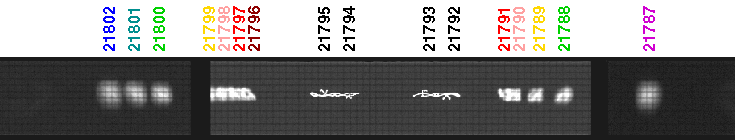
14 observations were made in March 2013 running from -21.3' to +24.75' (ObsIDs 15451-15464), typically for 1280 s, and another set of 16 observations in April 2019 that mostly filled in gaps (see Figure 15 right). The set of 16 (ObsIDs 21787-21802) used non-standard dither, 56"×40" with 1.7 ks exposures for most, and 128"×16"/2.4 ks for the 4 observations closest to the aim point. Telemetry was generally saturated--the source rate would be ~200 ct/s for observations on the thin-Al portion of the UV/ion shield--with a typical telemetered source rate of 120 ct/s and negligible background contamination within the source regions. Source rates on the thick-Al regions (ObsIDs 21793 and 21794, and parts of 21792 and 21795) were roughly halved. (The rate changes across the thick/thin Al boundaries on each side of the aim point were used to refine the boundaries' positions in a separate analysis.)
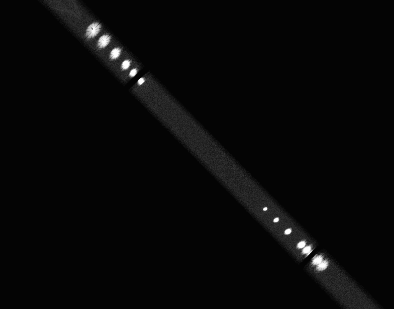
With the large pointing offsets required, the PSFs are broad and each observation covers several taps at once with a common broadband spectrum (see Figure 1) that extends well beyond the ~170 Å limit of LETG coverage. Using abc notation for each 1/3 of a tap, coverage of U taps (short axis) extended from 6a to 10a for the outermost dozen observations. Background contamination in the source PHDs is tiny and the associated errors in median pulse height are negligible, so we omitted background subtraction (which suffers various complications such as varying roll over the course of each observation set, making it difficult to extract identical source and background regions in detector coordinates).
 |
|
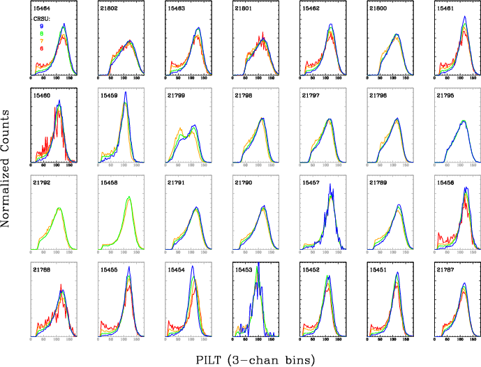
The broad PSF and large number of source counts of these observations provide an opportunity to study how gain varies in the cross-dispersion direction (CRSU, CHIPX, RAWX). Figure 16 compares PHDs for 8 representative ObsIDs broken down by CRSU. In all cases, the relative strength of the low-channel shelf increases toward low CRSU. The cause of this behavior is unknown (perhaps related to the MCP top-plate pore angle orientation, and/or nonuniform response to very-long-wavelength photons that are normally excluded by the grating) but it is not because of variations in the incident spectrum as a function of CRSU caused by a transition from the thin to thick Al coating on the UV/ion shield (see lab calibration C-K image). The top of the thick-Al "T" begins about 1/3 of the way onto the CRSU=10 tap, and even after accounting for the converging cone of focused X rays (half-angle ~3.4° for HRMA shell 1) which hits the UV/ion shield about 12 mm above the microchannel plates, any photons passing through the top of the T can only reach as as the very upper edge of tap 9.
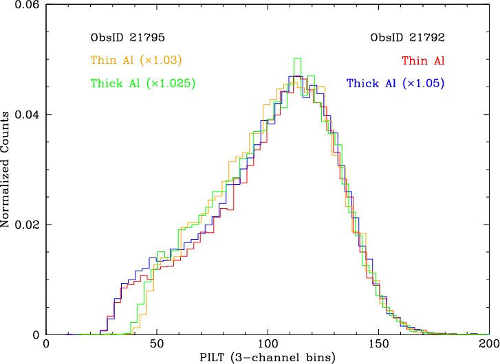
As noted above, source rates on the thick-Al area of the UV/ion shield are about half the thin-Al rates because of absorption, which is strongest just short of the Al-L edge at 170 Å (73 eV). PHD medians are essentially independent of wavelength for λ>70 Å (see Figure 9) but we investigated whether the PHD shape might differ on the thin- and thick-Al sides of the boundary (also being careful to use data from RAWX=2120-2170 [CRSU=8.28-8:48] given PHDs' dependence on CRSU--see Figure 16). As seen in Figure 17, there is no significant difference.
|
|
| Fig. 16: [pdf] PHDs as a function of CRSU for all but the 2 innermost of the 30 off-axis no-grating HZ43 observations, ordered by Yoffset from Plate 3 to Plate 1, with Plate 2 plots outlined in gray. Low-channel shelves generally grow stronger toward smaller CRSU, for unknown reasons. (The double peak for ObsID 21799 results from a since-corrected error in editing the gain coefficient for plate-edge subtap 125c, which has only a few pixels and should use the coefficient for 125b.) | Fig. 17: [pdf] PHDs on either side of the thick/thin Al boundary on the UV/ion shield, on both the - (ObsID 21795) and + (21792) wavelength sides. After adjusting for small differences in gain (×1.03, etc.), there is no significant change in PHD shape across either boundary. |
Might the increasing strength of the low-channel shelf with smaller CRSU seen in these special observations be something to worry about with standard dispersed LETG spectra? This could be answered by analyzing dispersed spectra that are offset in Z onto small CRSU, but we are not aware that any such data exist. (ObsID 9617, of Sirius B, was made with an offset that placed it onto CRSU=9-10.)
In any case, the observed dependence on CRSU is not likely to be a problem for LETG/HRC-S observations because: 1) dispersed spectra are much narrower in CRSU than most of these no-grating off-axis observations; 2) we are primarily using these data to calibrate relative gain along CRSV, and the shelf behavior appears to be fairly consistent as f(CRSV); 3) our calibration extracts data from CRSU/RAWY ranges that correspond to those covered by standard dispersed spectra (mostly on tap 8), where PHDs have weak low-channel shelves and little dependence on CRSU (see Figure 16 and discussion below).
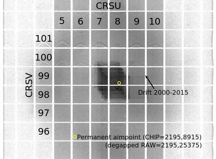
After applying TGAIN corrections and creating the PILT column, all 30 source event files can be merged and then treated like the other (dispersed) source data, extracting PHDs by CRSV subtap and computing medians, etc. To reduce systematic errors we choose a common range of CRSU for data extractions, one that approximates the range of dispersed spectra. Although the HRC-S aim point has drifted over time (Figure 18), and is now adjusted on a continual basis to fall near RAWX=2195 (CRSU=8.57), the average source position over the course of the mission is roughly RAWX=2175. The standard 40" dither pattern is 304 pixels wide, and adding another 23 pixels (Δtg_d=0.001 deg) on each side to enclose dispersed spectra at long wavelengths yields a range of roughly RAWX=2000-2350, or CRSU=7.81-9.18. PHD medians are fairly independent of CRSU over that range (Figure 19), so even highly nonuniform distributions of X-ray events on the detector during our calibration observations should not cause significant systematic errors.
|
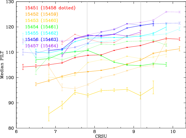
|
| Fig. 18: Cumulative exposure image in RAW coordinates for the HRC-S around the aim point (0th order for LETG spectra), showing the permanent aim point (implemented in 2016). | Fig. 19: [pdf] Median PILT for the first 14 off-axis HZ43 observations, by CRSU subtap. Thin gray vertical lines mark the ranged used (RAWX=2000-2350; CRSU=7.81-9.18) for sampling data when calibrating gain by CRSV subtap. |
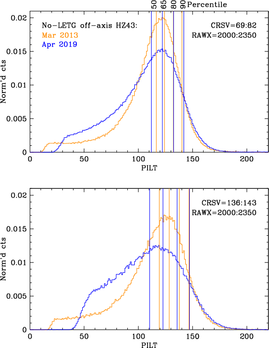
One additional concern, however, is whether changes in PHD shape, especially for low energy photons in low gain regions of the detector, have a significant effect on the consistency of measurements when using a mix of older and more recent data. In Fig. 19 we compare PILT PHDs from 1999 and 2019 LETG/HRC-S observations of HZ43 over the range CRSV=10-20, where gain is especially low (see Fig. 6). Fortunately, shapes at higher percentiles, where background filtering is applied, are very similar.
PHDs for HZ43 data without a grating, however, are broader and as shown
in Fig. 20, their shapes changed significantly over 6 years, so
that even though TGAIN rescaling yields consistent medians for
dispersed photons at a given position, medians for the no-grating
HZ43 observations are not consistent. Shapes in higher
channels are much more similar, however, and Fig. 21 illustrates
how we chose to use the 82.5th percentile as our metric.

|
|
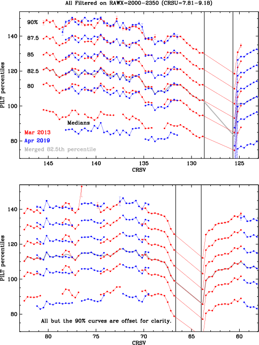
| Fig. 19: [pdf] Comparison of PHDs from LETG/HRC-S observations of HZ 43 early in the mission and recently, i.e., at high and low gain, from spectra in the lowest-gain region of the detector. Shapes are pretty similar, especially at high channels where background filtering is applied. Differences at low channels are from the increasing loss over time (as gain decreases) of events that fall below the detection threshold (before channels are rescaled to create PILT). | Fig. 20: [pdf] As noted above (Figs. 16 and 17 and in the text above), PHDs for the no-grating off-axis HZ43 observations are generally broader than for grating spectra, with excess events at low channels. Distortions are more pronounced at lower gains, leading to significant differences in PHD shape between the 2013 and 2019 data, so that medians at a given location are not consistent. | Fig. 21: [pdf] Various PILT metrics from the no-grating off-axis HZ43 observations. Because of changes in PHD shape (Fig. 20), medians did not provide consistent results between the two sets of observations (14 in 2013 and 16 in 2019). Based on the best overall agreement, an average of 80th and 85th percentiles was chosen to use for the combined data. |
Like the plate-gap regions, the area around the aim point has steeply decreasing gain (see Fig. 14/center). Although the no-grating HZ43 observations do not cover that range, there are several off-axis LETG observations of the emission-line source, Capella, that can be used to map gain, and those measurements can then be tied to the no-grating HZ43 measurements where they overlap.
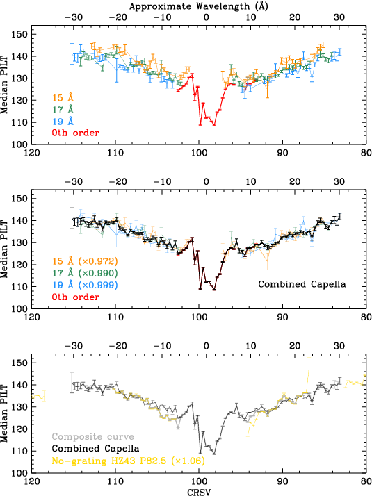
For this analysis, we again use data collected with a constant spectrum to provide "flat-field-like" calibration. The specific ObsIDs are: 1248, 58, 14240, and 18363 at Yoffset=0' (with some scatter in the coverage of CRSV because of aim point drift); 13090 at -0.75'; 6472, 3479, 2572, and 10600, at ±1.5'; and 5041 and 6165 at ±3.0'. The Capella spectrum is nearly constant over time, so 0th order can be used to provide one set of flat field data; other sets use specific bright emission lines. We extract circles or ellipses around 0th order and the lines at 15.02 and 16.78+17.05+17.10 Å (all Fe XVII), and 18.96 Å (O VIII Lyα), group the data by wavelength, extract PILT PHDs, and compute medians. A Yoffset of 1' corresponds to a shift of 3.36 Å (1.78 CRSV taps), and the standard 40" dither pattern covers 1.19 taps, so collectively those data cover a nearly continuous range from CRSV=83 to 114 (see Fig. 22).
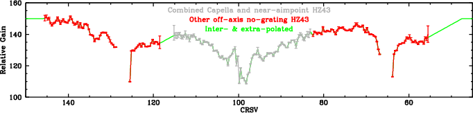
As seen in the top panel of Fig. 22, medians for each group of lines are slightly offset because of the difference in photon energy (or effective energy for 0th order). To combine the results we applied χ2 minimization, holding the 19 Å curve fixed while the 15- and 17-Å curves were adjusted, and then minimized that combined group's differences versus 0th order over the small range where they overlap. The resulting combined Capella curve is shown in the middle panel. (The large up-and-down pattern for taps 99-101 is seen in ObsIDs taken years apart, and therefore appears to be real.) These measurements overlap with some of the HZ43 measurements, which were similarly rescaled to match (Fig. 22 bottom panel). The composite curve (gray) is an uncertainty-weighted average of the Capella and HZ43 curves.
Agreement between the Capella and HZ43 data is not as good as between the various sources in Fig. 14, probably for the following reasons:
|
Fig. 22:
[pdf]
On- and off-axis Capella data used for gain "flat fielding."
Top: Medians from Capella 0th order and bright lines. Middle: Rescaled medians and combined curve for Capella. Bottom: Combined Capella curve and overlapping no-grating HZ43 curve (rescaled to match), with composite curve. |
|
| Fig. 23: [pdf] Composite gain curve from bottom panel of Fig. 22 and the other off-axis HZ43 measurements. Points are interpolated in gaps (CRSV=82c, 115b-118a) and estimated on the outer plates. |
|
The resulting combined HZ43+Capella calibration curve, with approximations for taps not covered, is shown in Fig. 23. In the next step, we use it to rescale the gains derived from LETG spectra, which smoothes out the major bumps seen in Fig. 14 and brings the overall shape close to its true PI vs λ form.
We apply the gain measurements from above by dividing the curve in Fig. 23 by 150 (i.e., normalizing to 1 at long wavelengths) and then calculate a new version of PILT with Spatial correction #1 as PILTS1 = PILTS/Normalized-Flat-Field-Curve. PILTS1 medians are calculated for each source, corrected for Higher Orders and 0th order position variations, and then averaged (with error weighting) to yield the composite medians. Results are shown in Fig. 24.
|
|
Fig. 24:
[pdf]
Top: PILT medians after Higher Order corrections (as in bottom
panels of Fig. 14).
Bottom: Error-weighted multi-source averages of PILTS1 medians. Exponential red and logarithmic blue curves illustrate possible models for fitting. |
The PILTS1 rescaling in Fig. 24 produces a noticeably smoother and more monotonic relationship of PHD median vs λ than for PILT, largely removing the gain sag near the 1/2 and 2/3 plate gaps, but some unexpected or inconsistent features remain. The dip and overcorrection between -2 and -8 Å can be fixed if we use only the off-axis Capella results (Fig. 22) and ignore the HZ43 scan; we do this in the PILTS2 scaling below. There is also an apparent overcorrection around CRSV=117-125 and probably CRSV=52-60.
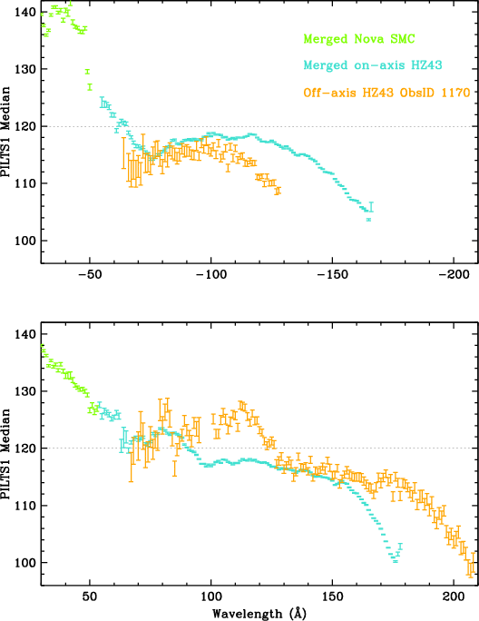
The most obvious remaining problem with the spatial calibration, however, is the gain droop toward the outer edges of Plates 1 and 3, beyond the range covered by the Capella/no-grating HZ43 flat fields. That range can be calibrated, somewhat indirectly, by analyzing ObsID 1170, a 10-ks LETG/HRC-S observation of HZ43 made with Yoffset=10'. That offset corresponds to 17.80 taps, or a shift of 32.9 Å, allowing one to compare PHDs from a given wavelength at two widely separated locations on the HRC-S.
For this analysis we analyze in wavelength space with 1 Å bins (a little over half a tap) and compare PILTS1 medians from the merged on-axis HZ43 spectra (and merged Nova SMC spectra at shorter wavelengths) with those from the off-axis ObsID 1170. The objectives are to make the on- and off-axis median vs. λ curves overlap by adjusting the gain coefficients, and also achieve consistency between + and - order spectra. Data extraction regions were adjusted because of the broadened off-axis PSF: the spectral region was offset by 5 pixels toward higher tg_d, and its half-width was increased by adding 51.5 pixels in quadrature with the on-axis region's half-width; background regions used the same shape as spectrum but were offset to the sides of the spectral region by 132 pixels instead of 85.
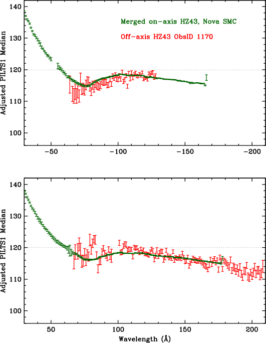
Figures 25 and 26 show results before and after the gain adjustments. The process is done by hand one subtap at a time, and is somewhat iterative and subjective, but converges naturally to yield gain coefficients that should be fairly accurate. As an example, in Fig. 25, the bump in the on-axis-observation curve around +70-95 Å is tied to the off-axis bump around 100-125 Å; both ranges correspond to CRSV of 61 to 49.
|
|
| Fig. 25: [pdf] PILTS1 medians for on- and off-axis spectra. The curves do not overlap because of incorrect relative gains on different areas of the detector. | Fig. 26: [pdf] Like Fig. 25 but after gain adjustments. |
The modifications to the PILTS1 scaling are used to create the PILTS2 scaling; a comparison of the two is shown in Fig. 27. As can be seen, a significant fraction of the PILTS1 corrections derived from the off-axis no-grating HZ43 observations is undone by the PILTS2 adjustments, although the two scalings are fairly close on Plate 3 (high CRSV). As discussed above, it is not clear what the problem is with the no-grating HZ43 data used to create the PILTS1 gain adjustments, but it may have something to do with very low energy photons that are dispersed off the detector when using the LETG.
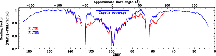
|
| Fig. 27: [pdf] Comparison of scaling coefficients to create PILTS1 (derived from the flat field Capella and HZ43 data) and PILTS2 (to achieve consistency between the off-axis HZ43 ObsID 1170 and on-axis data). PILTS2 scaling uses only Capella data near the aim point, after problems were noted in PILTS1 results based on the HZ43 scans. |
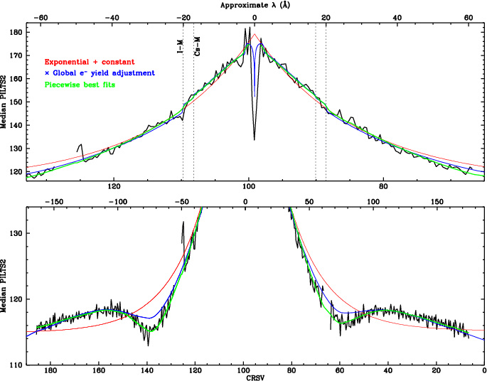
The new scaling is then applied to create PILTS2 from PILT, PHDs are extracted, and medians computed. Results are shown in Fig. 28. The next step in creating the final spatial gain map is to remove the residual deviations from a smooth curve. We find that an exponential plus a constant (red curve in the figure) roughly follows the data, but there appear to be relatively steep changes around the I-M absorption edge at 20 Å (most clearly seen in RS Oph spectra) and perhaps the Cs-M edge around 17 Å, as well as a deviation from monotonic decline centered around 75 Å. In our 2008 work we noted that the electron yield of the CsI photocathode showed related features (Fig. 29), and that an empirical correction factor based on the yield produced a better fit to the data. We therefore do piecewise fits over partially overlapping spans of ~25 taps at a time using an equation of the form
Median=YA (B e-|(99.12-CRSV)|/C+D)
where Y is the electron yield at the wavelength corresponding to tap CRSV, and typical coefficient values are A=0.014, B=64, C=15, and D=115. The fit results are then combined to yield the green curve in Fig. 28. (The fits used a slightly smoothed version of the CsI electron yield curve to account for dither, which smears out spectral features. The blue curve in Fig. 28 shows the best fit with a single set of parameter values on either side of 0th order, and uses the unsmoothed electron yield to better show effects at the absorption edges. Note also that the electron yield adjustment qualitatively reproduces the gain decrease observed at the very shortest wavelengths near the aim point; dither broadens the feature in CRSV space.) To remove the remaining small-scale gain variations we divide measured medians by the smooth model, and apply those final corrections to create the spatial gain map that is used to convert PILT to PI.
|
| |
| Fig. 28: [pdf] Median PILTS2 vs CRSV, with various smooth curves. An exponential plus constant (red curve) follows the general shape. Adding a term based on the CsI photocathode's electron yield (Fig. 29) improves the fit; the blue curve shows best fits to the + and - orders (fitted separately). The green curve is a composite of results from fits over spans of typically 25 taps. |
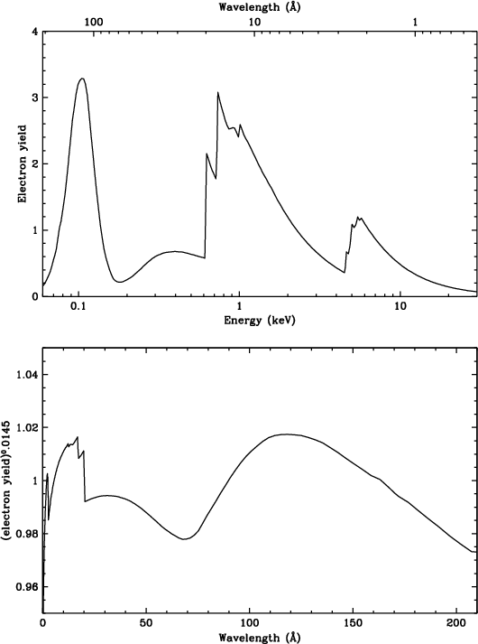
Fig. 29:
[pdf]
Top: Modeled electron yield of CsI. Bottom: Electron yield raised to the power of 0.0145 (typical for the fits used to create the green curve in Fig. 28) versus wavelength. Compare with the gain enhancement around 20 Å seen in Fig. 28, and the dip around 70 Å. |
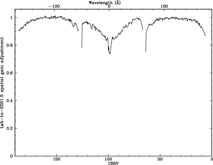
The collective spatial gain adjustments to convert from PILT to final PI are shown in Fig. 30. Adjustments near the plate gaps are especially abrupt, and as noted before, calibration uncertainties there are in general larger than elsewhere.
Fig. 31 plots total gain as a function of both position and time. Fig. 32 adds the effects of photon energy on pulse height to yield median SAMP values for dispersed spectra. Since the beginning of the mission, the lowest PHDs have been generated for CRSV lower than ~30, corresponding to positive wavelengths longer than ~130 Å, but within the next couple years, the region around CRSV~130-140 (λ~60-80 Å) is expected to reach similarly low pulse heights. The effects of low-channel losses on PHD shapes will become increasingly severe, but can in principle be calibrated. The rate of QE decline will also accelerate, and will likely be the dominant factor in deciding when/if to raise the HRC-S high voltage.
|
|
|
| Fig. 30: [pdf] Collective adjustments for lab-to-2001.5 gain changes. (2001.5 is the reference date for TGAIN corrections, chosen because the overall flight gain at that time is closest to the lab gain.) | Fig. 31: [pdf] Inverse GAINMAP coefficients (for CRSU=8a subtap) times TGAIN scaling, illustrating relative gain as f(CRSV,time). | Fig. 32: [pdf] Modeled median SAMP for dispersed 1st order spectra, calculated using model PI medians (green fitted curve in Fig. 28) multiplied by the scaling coefficients in Fig. 31. Compare with measurements from flight data in Fig. 6. |
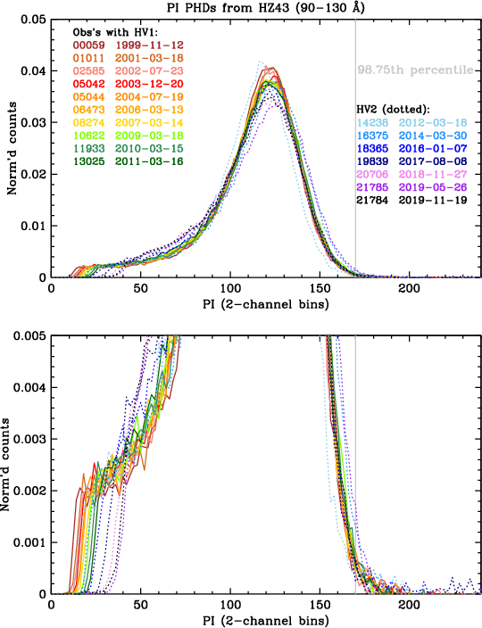
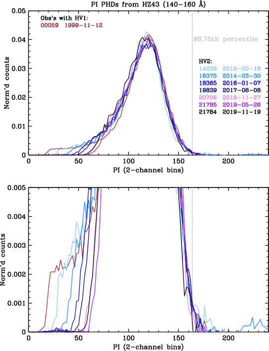
The ultimate purpose of this gain calibration is to allow processing of LETG/HRC-S data so that pulse height filtering can be applied, resulting in substantial background reduction with the loss of a very small and well determined fraction of X-ray source events. This requires that the shape of PI PHDs remains essentially constant over time, particularly at the high channels where filtering is applied. Figures 33 and 34 show the PI PHDs in two long-wavelength ranges from selected HZ 43 observations over the course of the mission. Three features are of particular note:
|
|
| Fig. 33: [pdf] PI PHDs for 90-130 Å in HZ43 observations typically 1.5 years apart. Note the rising low-channel cutoff and gradual widening of the peaks with lower gain. Raising the high voltage largely restored the PHD shape. PHD shapes at high channels have little sensitivity to gain. | Fig. 34: [pdf] PI PHDs for 140-160 Å, currently the lowest-gain region of the HRC-S. For clarity, only one observation with HV1 is shown. |
To determine the appropriate filtering limits, we extracted 1-Å bins from the merged source event files and computed PI medians and high percentile metrics (97.5th to 99th). HO corrections, which were derived for PHD medians, were applied for all metrics. Generally they worked well, but judging from ranges where pure 1st order spectra overlapped with those having some HO contamination, high-percentile results sometimes had significant errors even when HO contamination was fairly small. At each wavelength we therefore used results from the source(s) with the smallest total uncertainty in the median, with minimal overlap. Results were then averaged, yielding the results in Fig. 35.
The high-percentile curves show a clear periodic structure at long positive wavelengths, and similar though less regular structure on the negative side. The period is about 15 Å, which corresponds to 8 taps, a periodicity that is not uncommon in HRC-S data. Another complication is that, by grouping observations and using large wavelength bins, there are signs of systematic changes in high-percentile metrics at some long wavelengths where PHDs are most susceptible to distortions caused by low-channel event loss. In the 2008 calibration, it was decided that using the 98.75th percentile curve for filtering provided the best compromise between background removal and X-ray event retention, but given the indications of recent PHD distortion at very low gains, we have adopted slightly more conservative filtering limits (the top black line in Fig. 35), aiming for 1% X-ray event loss instead of 1.25%.

|
|
|
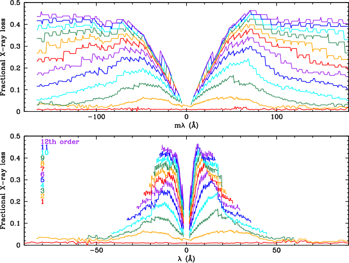
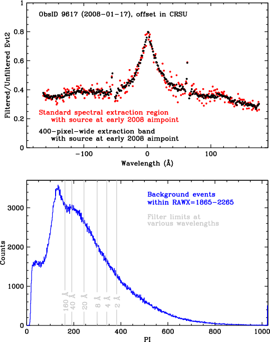
| Fig. 35: [pdf] Curves for the PI median and 97.5th to 99.0th percentiles. Top black curve denotes the PI vs tg_mlam filter, removing approximately 1.0 [0.8-1.5] percent of Level 2 X-ray events. | Fig. 36: [pdf] Effect of filtering on orders m=1-12. Curves are higher than in actuality from ~12 to 17 Å because of small but increasing HO contamination in the Mkn 421 data used out to |λ|=17 Å; there is no real jump between 17 and 18 Å. The small step around 20 Å, however, is real and is caused by an increase in gain at the I-M absorption edge (Figs. 28 and 29). The jump around 2 Å is also from photocathode absorption edges. | Fig. 37: [pdf] Effect of filtering on pure background in or near the spectroscopy region. Top: The most effective filtering is at long wavelengths, where events beyond PI~160 are removed (see Fig. 35). Bottom: Background PHD, with filtering limits at selected wavelengths. |
The 1% event loss is for the 1st order spectrum. Losses are progressively larger for higher orders, which have PHDs shifted to higher channels. Using the PHDs extracted from ~pure 1st order spectra, we applied the PI filter limits (for Å) to the PHDs for Å/m to determine the effect on mth order. Results through 12th order are shown in Fig. 36. Small losses of higher order flux will usually be unimportant, but observers can use Fig. 36 to estimate the effect of filtering on HOs and adjust their spectral fitting models accordingly.
To quantify the effect of filtering on background events we use data from ObsID 9617, in which the source was offset from the standard aim point by nearly 2 CRSU taps, leaving the standard spectroscopy region free of X-ray events. We extracted events from that region, applied the filter, and computed the fraction of events that remained after filtering (red points in top panel of Fig. 37). To obtain better statistics, we did the same analysis using a wider extraction region (black points). 60-70% of evt2 background events are removed at |λ|>40 Å, falling to ~20% removal at the shortest wavelengths.
The particle background varies over the solar cycle (see POG Fig. 9.21.) ObsID 9617 was collected in 2008, when the solar cycle was near its minimum, background rates were near their peak, and the cosmic ray energy distribution near Earth was somewhat harder (with relatively more background events at high channels) than at solar maximum. The background filter effectiveness shown in Fig. 37 therefore represents the best case. The fraction of background events that are removed by the filter near solar maximum (next expected ~2024) is a little lower, but the absolute background rate is also lower.
The current TGAIN calibration runs through fall 2022, but can be extended by adding more epochs and extrapolating the current fits, or by analyzing new data and making new fits. It is not unlikely that the detector high voltage will be increased within the next few years, which will of course require new TGAIN data. The decision on when to raise the voltage will be driven mostly by consideration of the decreasing QE.
At some point it may become necessary for TGAIN calibration to be adjusted to take into account differences in the temporal behavior of the median versus the 99th percentile. With so few counts per channel at high percentiles, it is difficult to detect trends, but this can be overcome by grouping observations and using large wavelength bins. Such an occasion would also provide the opportunity to calibrate the 8-tap periodic structure seen at high percentiles in Fig. 35, which would allow slightly tighter and more effective filtering.
Whenever the next calibration is done, there are a few additional improvements to consider:
Last modified: 06/16/20


![[png]](./sampleBy3plate1Uncorr.png)
![[png]](./sampleBy3plate2Uncorr.png)
![[png]](./sampleBy3plate3Uncorr.png)