
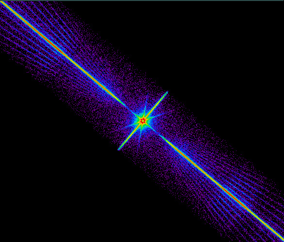
The LETG/HRC-S spectral extraction region has a 'bow tie' shape, narrow in the middle and widening on the outer plates to accommodate the inherent astigmatism of the LETG's Rowland-circle geometry. The shape and size of this region were chosen early in the mission based on MARX simulations (see Fig. 1) to roughly optimize the tradeoff between inclusion of X-ray signal versus particle background. The work described here re-optimizes the spectral extraction region based on observational data, and recalibrates the enclosed energy fraction (EEFRAC). As described below, the true spatial distribution of the dispersed spectrum differs in several small but sometimes significant ways from the ideal:
Together, these effects can add up to deviations of more than ± 6 pixels in the tg_d direction near the plate ends, although errors are more typically 1 or 2 pixels. For comparison, the current extraction region half width is 12.45 pixels (80 μm, 5.31e-4 deg) in the central region. At 170 Å the half width is 42.1 pixels (270.7 μm, 19.96e-4 deg).

|
|
| Fig. 1. MARX simulation (c. 2000) of a flat spectrum illustrating the broadening of the LETG/HRC-S profile in the cross-dispersion direction toward longer wavelengths, and showing the standard bowtie extraction region. Vertical axis is stretched by a factor of ~220. | Fig. 2. Image of combined HZ43 spectra, after removal of tilts and wiggles (see below). Vertical axis is stretched by a factor of 200. The white horizontal line marks the median of the cross-dispersion profile, which is visibly asymmetric. See also Fig. 11 below. |
The intention of this analysis is to straighten and align dispersed spectra, and then calibrate the intrinsic cross-dispersion profile as a function of wavelength. We can then define a narrower spectral extraction region that yields higher S/N.
We use bright, frequently observed continuum sources to provide complete wavelength coverage with high signal, principally Mkn421 and PKS2155 for short wavelengths (<~60 Å) and HZ43 for longer wavelengths. All the observations we use were made on-axis (Yoffset=0) and were processed to Level 2 using the latest CALDB. The LETGS Background Filter was applied and time periods with DTF<0.98 (indicating significant background flaring) were removed to improve S/N. Another reason to remove flares is that HRC background is spatially nonuniform during those times, with crowning across the short axis and shadowing by the thicker Al coating on the "T" portion of the uv/ion shield.
Our analysis first concentrates on individual observations, measuring and correcting the 0th order position, spectral tilt, and tg_d offsets. The corrected event files are then combined into a single file for each source; data from two other sources (RS Oph and KT Eri) receive the same treatment and are included in the EEFRAC analysis. Those results are then used to calibrate extraction efficiency as a function of wavelength and extraction region width, and to determine how wide the region should be to optimize S/N.
The CIAO tool celldetect is used by tgdetect in Standard Data Processing to determine the position of 0th order, which is then used as the origin for the grating coordinates tg_d and tg_r. Errors of a few tenths of a pixel in 0th order are common in Archive data. As described in more detail below, a refined 0th order position can be obtained by iteratively applying dmstat to find the mean x and y values using a circle of radius 12. The improved position is then used as an input to tg_create_mask, followed by processing to Level 2.
After reprocessing each observation using new 0th order positions we extracted tg_d profiles for each dispersion-axis tap (crsv) with the assumption (consistent with analysis of a few off-axis observations) that profiles are, over short spatial scales, predominantly a function of location along the detector rather than a function of wavelength. Binning by tap typically provides a few thousand events (and thus centroiding errors of a couple/few percent of the profile FWHM) and good sampling of the dispersed spectrum's wiggles. Within a tap, tg_d is binned by 0.00005 degrees (~1.2 pixels) on the central plate and 0.00007 to 0.00010 degrees on the outer plates where the profiles are wider (see Fig. 1). Wider bins may obscure detail while narrower bins may have too few counts, causing interpolation errors.
The findcenter.f program reads the tg_d profile data for each tap, determines and subtracts the background level, and computes the median tg_d with interpolation between bins for greater accuracy. Background is determined using tg_d ranges beyond the main profile wings and that avoid cross-dispersed orders (discussed in more detail below). To remove the initially uncalibrated wiggle (see below) from our results and enable a better determination of the relative tilt of each spectrum, the average tg_d median is computed as f(crsv) for all the observations of a given source and then subtracted from the individual median for each ObsID. Results, grouped by source, are shown below. Emission lines from Capella, a bright coronal source, were used to help tie together the short- and long-wavelength calibration.
|
|
|
|
| Fig. 3. tg_d medians vs crsv, after subtracting the average tg_d median for each source. Tilts are therefore relative to the average tilt for each source. For continuum sources, only points with errors of less than 1e-5 degrees (about 1/4 pixel) are plotted. Errors for Capella's lines' medians are explicitly shown. Labels list ObsID and observation date (yymmdd). | |||
As can be clearly seen in the left-panel plots, LETG/HRC-S spectra have a time dependent tilt. (LETG/ACIS spectra presumably do too, but the extraction region is wider and the spectra shorter so the effects are negligible.) Right-panel plots show results after tilts are removed. Note that even after correcting the 0th order positions and tilts, some spectra (e.g., 3rd right panel for HZ43) have a general tg_d offset. This seems to be correlated with the time of year and may therefore be a thermal effect. There is also a slight time-dependent curvature, particularly on the inner plate (e.g., upward curvature for early Mkn421 observations and downward for later---see here). The earliest observations also show relatively large deviations in tg_d offsets and/or curvature near 0th order.
Within each source-group, tilts are well determined relative to the group average and we removed the tilt in each observation by running a python script that adjusts the tg_d value for every event in a given observation's event file. All the files for a given source were then combined using dmmerge in order to improve statistics. (The two weakest PKS2155 spectra were not included in that source's combined file.)
After removing tilts, a time-independent pattern of tg_d median versus crsv remains (Fig. 4), which also means that defining an absolute tilt for any one observation is somewhat arbitrary. Because of minimal wavelength overlap of the continuum sources, there is also some ambiguity in how tilts are measured on the inner versus outer plates. Capella spectra, which have prominent lines on all three plates, were analyzed to address the latter issue but relatively large measurement uncertainties (note error bars in Fig. 3) prevented a definitive calibration.
We therefore adjusted the tilts of the four composite spectra by eye in order to obtain the best agreement among them (Figs. 4 and 5) and also added a 1.0-pixel global tg_d offset to make the wiggles roughly symmetric about tg_d=0 (Fig. 4). In the overlap region between roughly 80 and 100 Å, higher order diffraction contributes most of the events seen in the hard continuum source spectra, which broadens the tg_d profile and skews the median. We therefore ignore those results and use only data from HZ43. Higher order flux is also significant (20-40%) just short of the C-K absorption edge and between ~60 and 80 Å but the effects on the tg_d profile appear to be minor. Short of ~55 Å the results from HZ43 become increasingly suspect because of decreasing flux.
|
|
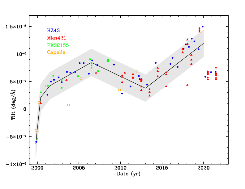
| Fig. 4. Median tg_d values for combined spectra, with tilt and offset adjustments to make the wiggle symmetric about tg_d=0. tg_d values are multiplied by 1000 for convenience and units are degrees. Tilts are in units of degrees per tap, also multiplied by 1000. Legend example: blue points are for 18 combined HZ43 spectra, with a tilt correction of 0.00090 and offset of 0.029. The composite wiggle curve is shown in black; some points near 0th order and the ends of the inner plate were adjusted by hand because the true errors are larger than indicated by the purely statistical error bars. (Clicking on the figure shows a 2-panel plot; the lower panel plots the same data without the offsets, showing the net wiggle correction and residual scatter among the different source curves.) | Fig. 5. Time dependent tilts in deg/Å. Uncertainties on each point (excluding Capella) are small, so the observed scatter is real and probably related to thermal conditions. There is no apparent correlation with aimpoint jumps. The solid black line can be used to estimate the tilt in most observations, and the gray band denotes the degree of uncertainty that would cause a 1-pixel error at 170 Å. (This figure is updated roughly once a year.) |
With a consistent measure of tilt across all three plates, the tilt-versus-time curves from all 4 sources can be plotted together, as shown in Fig 5. The gray band represents a tilt uncertainty that would cause 1 pixel of error at 170 Å (and proportionally less at shorter wavelengths). Error bars on the points in Fig. 5 are quite small, so the jump between the blue HZ43 points around 2010 is real, as is the deviation from trend in 2014. The cause of these jumps and other scatter is unknown; there is no correlation with aimpoint jumps or any other parameters that we investigated.
After applying tilt and wiggle corrections to the combined data we can calibrate the tg_d profile, or cross-dispersion Line Spread Function (LSF), and define narrower spectral extraction regions to improve S/N. However, the hard-source spectra we use to calibrate spectral tilt and wiggles have strong higher orders which broaden the measured LSF and have their own cross-dispersion orders (see below). We therefore include observations of the very bright pseudo-continuum sources RS Oph (ObsIDs 7296, 7297) and KT Eri (ObsIDs 12097, 12100, 12101, 12203) in our analysis. First order covers 15-30 Å in RS Oph and 20-50 Å in KT Eri (see Fig. 6) and there is essentially no higher order contamination in those wavelength ranges. The observations we use were obtained when those sources were extremely bright, often exceeding the HRC-S telemetry limit. High rates can distort the core of the 0th order PSF but did not affect the LSF of dispersed spectra, except for the highest-rate portions of ObsID 12203 (23-35 Å; see Figs. 6 and 7) which we do not include in further analysis. DTF filtering, which was applied to Mkn421, PKS2155, and HZ43 data in order to eliminate periods of background flaring, was not applied to RS Oph or KT Eri data because that would remove data during the many periods of telemetry saturation and because background is comparatively negligible during those very-high-rate observations.
|
|
| Fig. 6. Spectra used for central plate. The combined Mkn421 spectrum has by far the most counts but had the lowest average counting rate, and therefore relatively more background. It also has the largest contribution of higher order diffraction. The KT Eri observation 12203 had the highest rate and its LSF was noticeably broader at some wavelengths than the others (see Fig. 7). | Fig. 7. Comparison of background-subtracted LSFs (tg_d profiles) around +25 Å. Residual errors of up to 1/4 pixel in tg_d centroid were corrected for these plots to enable easier comparisons (but not in the evt files because such errors are representative of what users can expect). The LSF of Obsid 12203 is broader than the others and we omitted its data between 23 and 35 Å from subsequent analysis. The other ObsIDs do not suffer from high-rate distortions, although the Mkn421 LSFs are broadened at some wavelengths by higher order contributions. |
We used data from KT Eri and RS Oph as described above, along with Mkn421 data between 5.5 and 8.4 Å. Rates shortward of 5.5 Å drop rapidly so that 2nd order contamination in our chosen range is very small, and 3rd order is even less. The large number of events in this data set (about 550,000 in 0th order) provides adequate statistics to see to mX=10, with hints of 11th order (Fig. 10).
|
|
| Fig. 8 (above left). Image of Xdisp orders, etc. Click on image for an explanation of the features. | |
| Fig. 9 (above right). Comparison of LSFs (25-40 Å) from KT Eri (orange) and Mkn421 (black). Because of higher order contamination, the Mkn421 profile is broader in the core and includes extra cross-dispersion peaks. (The distinct shoulders on the KT Eri profile between the core and the 1st cross-dispersion peak are from coarse-support-structure diffraction.) | |
| Fig. 10 (right). Cross-dispersion orders; profiles from - and + orders are combined. Large X's mark peaks not used for calibration because of uncertainties in the underlying wings of the main-peak LSF. + signs mark the region-of-interest boundaries on either side of a peak; interpeak ranges are used to determine the local background, which includes intrinsic HRC background and underlying counts from the wings of the primary order. Dotted line marks the detector background level. Mkn421 background levels were adjusted (- signs) as described in the text. | |
Event-file data were divided into thin triangular wedges (source center at pointy end) so that events of any given Xdisp order are collected together regardless of wavelength. Wavelength ranges for each source were chosen to provide optimal combinations of order coverage and S/N. Data from + and - primary orders and + and - Xdisp orders were combined, with the tg_d limit of ±0.021 deg chosen to maintain a flat detector background (i.e., without dither losses near the edges). Data were also analyzed separately (+ vs -) to confirm that results were the same within errors. Great care was taken to ensure that the dithered edges of the detector were excluded so that the background is linear over the tg_d range of interest.
As shown in Fig. 10 we were able to calibrate out to Xdisp order 10; distinct peaks out to order 12 were seen using Mkn421 data with λ=5.5-7.5 Å but uncertainties were large. The Mkn421 short-wavelength orders are so close together that their wings overlap and the local background levels can not be seen. We therefore adjusted them so that results for orders 3 and 4 matched those from RS Oph and KT Eri, scaling the background adjustments for each peak by its intensity. The net change was to increase each peak by about 5%.
A model using a sum of 3 squared sinc functions (appropriate for ideal gratings) was fit to the results for orders 1-10 and extrapolated to order 1000. Results are shown in the Table below. More discussion and a comparison with previous work from the the 1998 SRON Final Report on LETG calibration are provided in Appendix A. Based on our fits and the SRON report's caveats about PSF wings and background we believe that their results (using Al-K) are too high for orders 1, 2, and >10.
We find that Xdisp orders have a total of 9% as much flux as the primary order, vs. the 11% that would be expected based on a simple model using measured support-structure parameters. Xdisp relative intensities should be wavelength independent because the support structure is opaque over the energy range of interest, however we measured the intensity of order 1 as 0.84±0.01% of 0th order for λ=15-39 Å using data from RS Oph and KT Eri, and 0.76±0.04% over λ=70-82 Å with HZ43 data, a 2σ difference. Our final answer in the table below uses a weighted average of these results.
Order	Intensity relative to 0th, with statistical uncertainty
-----	-------------------------------------------------------
1	0.00831  0.00010
2       0.00781  0.00010
3       0.00678  0.00010
4       0.00569  0.00016
5       0.00405  0.00013
6       0.00316  0.00013
7       0.00191  0.00012
8       0.00113  0.00012
9       0.00086  0.00012
10      0.00046  0.00011
>10     0.0048   modeled
Total	0.0450 ±0.00041  * 2 for both sides = 0.0900±0.0008.
Appendix A: More details on Xdisp measurements and models.
As noted above, the intensity of Xdisp orders must be known in order to properly determine the background level, which is critical for measurements of the tg_d profile. For those measurements we first bin the profiles by 0.00005 degrees (~1.2 pixels) in 1-Å slices, within the range -0.0248 < tg_d < 0.0208 degrees, which avoids dithered-edge effects for all the observations under study. The program profilesBYang.f reads in each profile, determines tg_d ranges affected by Xdisp orders, and then computes the background on each side for |tg_d|>0.015 degrees after excluding Xdisp peaks. At shorter wavelengths, Xdisp peaks are so close together that little if any clear background range is left. In those cases the program iteratively computes the 0th order intensity after subtracting estimated background and Xdisp peaks (scaled from the 0th order intensity) and quickly converges to the underlying background. Comparisons of backgrounds derived using this method and the exclude-Xdisp-orders method in wavelength ranges where both could be used showed excellent agreement so we chose to use the scaled-Xdisp method in all cases. A linear background was then computed and subtracted, yielding clean tg_d profiles normalized to sum to 1 when including the intensities of Xdisp orders outside the tg_d range of analysis, i.e., 2π normalization.
Those profiles were read by eefrac.f, which boxcar-smooths the data by 3 Å; we tried several binnings and this gave a good compromise of S/N and wavelength resolution. The program then steps through each profile, summing the normalized intensities, and computing the tg_d value at various enclosed energy fraction (EEFRAC) values. Results are shown in Fig. 11a.
Close inspection reveals that the RS Oph and KT Eri contours are generally tighter than those for Mkn421 because of higher order contamination in the latter. This is especially pronounced just short of the C-K absorption edge where 1st order intensity is very low. Higher order contamination should be very small here for KT Eri (see Fig. 6) but contour deviations are still apparent; scattering from the central source (the primary 0th order) is probably also contributing.
The noisiness of the contours in Fig. 11a is partly statistical, but most of it comes from systematic errors in the background determination, presumably from faint off-axis sources and nonlinearities in the detector background, mostly in regions outside the plotted tg_d range, which is only about 10% of the 6-tap detector width. Errors in the background are usually from localized excesses, which pull the contours farther from the core than they should be. We attempt to correct for these errors and retrieve the true tg_d profile by forcing the outermost contours in our analysis, the 6% and 94% levels, to follow idealized contours. The fixeefrac.f program resets the cumulative profile intensities, eliminating most of the noise in the interior contours, and also adds output for more EEFRAC levels near the profile core. In the final version (Fig. 11b) we have drawn piecewise linear curves by eye to best match the results while taking into consideration errors from residual higher order contamination, etc.
| 
|
| Fig. 11a. Cumulative count fractions from four continuum sources. Overlapping data on the center plate are distinguished by line thickness. The cross-dispersion 1st order is shown in light gray (also seen as the faint "whiskers" in Fig. 1). Solid black lines mark the current spectral extraction region (bowtie). The red and magenta "Uncorrected" curves show the medians for two ObsIDs with extreme tilts (before correction--see Fig. 3). The gray band in the middle has a half-width of 1 pixel; typical deviations from a perfectly straightened spectrum (arising from errors in 0th order position, residual time-dependent spectral curvature, etc.) are ±0.5 pixels or less. |
Fig. 11b. "Corrected" version of Fig. 11a including more
contours in the LSF core and using only the best
data for the central plate, forcing the 6% and 94% contours
to follow their assumed true values,
and then drawing piecewise linear curves for all contours.
Contours short of ~6 Å are approximate;
final EEFRAC results at short wavelengths
incorporate MARX modeling of Xdisp orders and scattering.
Plots of intermediate steps:
|
As seen in Fig. 11, the cross-dispersion profile is asymmetric, with the tightest LSF in the lower left quadrant (- wavelength, - tg_d side). Another illustration is shown in Fig. 12. One can see in Fig. 11 that the bowtie follows contours corresponding to an 85-86% extraction efficiency on the outer plates but includes slightly more X-ray signal---and quite a bit more background than necessary---toward shorter wavelengths.
|
| Fig. 12. tg_d profiles (0.00002-deg = 0.47-pixel bins) for 10-Å slices of the combined HZ43 spectrum. LSFs for shorter wavelengths are shown in Appendix B. |
As seen in Fig. 12, LSFs are asymmetric about tg_d=0 and also differ at + and - wavelengths. The latter is initially surprising because the diffraction pattern from a given grating facet must be symmetric about 0th order. A discussion of possible causes, including what we believe must be the correct explanation, is presented in Appendix C.
The program SNcalcs.f computes the S/N ratios for spectral features of width 0.07 Å (the LETG FWHM resolution is 0.05 Å) having S0 counts collected (if EEFRAC=100%) in exposures of T seconds. Spectral extraction regions were made of paired contours from Fig. 11, e.g., the region between the 8% and 92% contours has an EEFRAC of 84%. S/N = (EEFRAC × S0) /((EEFRAC × S0)+BG)0.5 was computed for various combinations of S0 and exposure times. Note that lines and continuum emission were not considered separately and that the S/N of line features will be reduced when continuum is present. Background data were taken from the composite HZ43 and Mkn421 observations. Those data were collected over roughly a dozen years and therefore represent typical HRC-S background rates, which vary by roughly a factor of two over the solar cycle (see POG Fig. 9.21).
Results are shown in Figs. 13 and 14. As can be seen, as the background becomes a larger factor in the noise term, S/N becomes more sensitive to the choice of extraction region. Except in the case of short observations with strong spectral features (e.g.,upper left panel in both Figures) where the S/N is already large, one can always improve the S/N by using a narrower extraction region. An extraction region with EEFRAC~78%, which reduces the net spectral extraction efficiency by ~8% and reduces background by 45-55% compared with using the standard bowtie region, provides the best or nearly best results in most low-S/N cases.
| 
| 
|
| Fig. 13. S/N ratios for various combinations of spectral feature counts (S0 listed along the left for 100% extraction efficiency) and exposure time T (across the top). Within each panel, a family of S/N curves is shown for a range of spectral extraction efficiencies. (Plot for 25-141 counts.) | Fig. 14. Change in S/N compared with using the standard bowtie extraction region. The optimal extraction region varies slightly depending on exposure, number of spectral feature counts, and wavelength but S/N is generally at or near its maximum with EEFRAC=78%. (Plot for 25-141 counts.) | Fig. 15. tg_d midpoints of EE contour pairs (e.g., EEFRAC=78% curve is for the 11% and 89% contours in Fig. 11). Based on the S/N analysis we use the 78% curve as a final tg_d correction so that a symmetric extraction region can be used, thus avoiding complicated modifications to CIAO and the CALDB architecture. |
Because the LSFs are not symmetric we also examined the effect of using asymmetric pairs of contours, e.g., the 10%|88% or 12%|90% contours instead of the symmetric 11%|89% pair to obtain EEFRAC=78%. We find that shifting the extraction region by ~1 pixel, corresponding to a change of a couple or few percent in the EE contours, has only a tiny effect on the net S/N.
Spectral extraction efficiencies are tabulated for each combination of detector (ACIS-S or HRC-S) and 1st order (+ or -) in the EEFRAC block of the corresponding CALDB LSFPARM file (see here). For HRC-S, wavelength runs from 0 to ±184.23 Å in 2048 steps of 0.09 Å, with 10 values of |tg_d| (now increased to 23 to better capture the LSFs' structure). The existing CIAO/CALDB architecture implicitly assumes that the LSFs are symmetric. To work within that system we therefore apply a final tg_d correction to our calibration data, a wavelength dependent offset that makes the 11% and 88% contours of Fig. 11 (yielding EEFRAC=78%) symmetric about tg_d=0 (see Fig. 15).
To populate the table data with EEFRAC(Å,tg_d), where tg_d is the full width of the extraction region, we begin with the original 10 tg_d values and interpolate from our EEFRAC measurements wherever possible, which is between the EEFRAC=88% curves (the 6% and 94% contours in Fig. 11b) and with |λ| > ~13 Å. Our measurements do not adequately cover shorter wavelengths so there we rely on the previous CALDB results which are based on raytrace simulations, rescaling them to account for the lower Xdisp intensities (totaling 9% instead of the previous 11%) and renormalizing to the 2π flux instead of flux within the effective detector area. Fig. 16 shows that this approximate rescaling works reasonably well, although a second-order rescaling is needed to make the simulated EEFRACs smoothly join with the measured EEFRACs at ~13 Å (see Fig. 17). The 2nd order scaling factors for the three smallest tg_d values are 1.065, 0.986, and 0.972, respectively. Beyond the 6% and 94% contours we use the old EEFRAC values with just the first-order rescaling. The remaining tg_d/wavelength parameter space is filled by drawing straight lines to connect the measurement- and simulation-based data (Fig. 17). The dotted curves are conservative—EEFRACs are probably a bit lower than reality—but the practical effects are negligible because those curves only come into play when extraction regions are much wider than the standard bowtie.
Interpolation errors using only 10 tg_d values can exceed 1% at some wavelengths using the standard bowtie extraction region and several percent if using a narrower region so we added another 13 tg_d values to the EEFRAC table. Again, most of these new array elements were populated by interpolating from our finely sampled measurement data. At short wavelengths we rescaled EEFRAC values from the nearest one or two of the 10 original tg_d values to smoothly join with the measurement-based values. Final results are shown in Fig. 18.
The resulting EEFRAC tables, which will were implemented in CALDB version 4.6.9 on 23 Sep 2015, are, strictly speaking, only appropriate when the full complement of tg_d corrections (tilt, wiggle, and symmetrization) is applied to the data, as should be done whenever a narrow extraction region is used. Errors in the derived EEFRAC are, however, negligible when using standard processing data (i.e., with the standard bowtie extraction region, without any tg_d corrections).
| 
| 
|
| Fig. 16. EEFRACs for the standard bowtie extraction region using data from the old CALDB data (red), roughly rescaled CALDB data (orange), calibration measurements (blue, using data from Fig. 11e), and new CALDB (black). The ratio of new and old CALDB EEFRACs (and the inverse of new/old HRC-S QE) is shown in gray. | Fig. 17. New EEFRAC values for the ten original tg_d values. Values interpolated from calibration measurements are plotted with thick lines, those based on rescaled old CALDB data (from raytrace simulations) are thin (at short wavelengths). Dotted connecting lines follow trends in the old CALDB data. | Fig. 18. Final EEFRAC curves for the complete set of 23 tg_d values, with the 13 new curves shown in black. |
The EEFRACs from this work differ from those in the previous version of the CALDB because of deviations from the simulated LSF, 2% lower Xdisp intensity, and the previous incorrect normalization of flux to the detector area rather than to 2π. The net change in bowtie-region EEFRACs is typically several percent, and about 12% at the longest wavelengths (Fig. 16). Note that the overall absolute uncertainty in the LETG/HRC-S EA is unchanged at approximately ±10% (somewhat larger at long wavelengths because of complications from recent changes in HRC-S gain and QE).
Systematic uncertainties in the background are believed to be the largest source of error in the present work, particularly at short wavelengths where high-energy scattering is largest and support-structure diffraction from 0th order leads to some unavoidable ambiguity in what constitutes the effective background. While difficult to estimate we believe that when using the standard bowtie extraction region the net error of this analysis is of order 1-2% but probably a bit larger short of λ~10 Å. There may also be small systematic differences in effective EEFRACs between line-dominated and continuum sources because of differences in the relative contribution of scattered and Xdisp flux from adjoining wavelengths.
The lower total Xdisp intensity, measured as 9% of the main order intensity vs the old 11%, is difficult to understand from a theoretical perspective given the relative simplicity of opaque-bar grating models. One possibility is that imperfect manufacturing and/or assembly has redistributed the missing power to orders beyond our calibration rather than removed it.
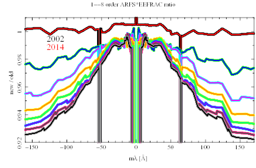
Despite these changes in the EEFRAC calibration, the net LETG/HRC-S effective area (EA) for 1st order remains unchanged. This is because the EA, which includes the bowtie EEFRAC and HRC-S QE as factors, is calibrated by comparison with theoretical model spectra of Sirius B and PKS 2155/Mkn 421, so that any changes in EEFRACs are compensated by corresponding inverse changes in detector QE. CALDB changes resulting from this work are therefore transparent to users of LETG/HRC-S data unless they are using an extraction region narrower than the default (in which case the exact Xdisp profile is important, but even here differences in net EA will usually be no more than a few percent) or unless they are analyzing spectra where higher order diffraction is important. In the latter case, the accompanying changes in HRC-S QE (see gray curve in Fig. 16), combined with calculation of higher order gRMF EEFRACs based on mλ (rather than λ, as for the QE), mean that net EA for very high orders may be up to ~12% lower than before at the largest values of mλ (see plot comparing old vs. new effective areas for orders 1 to 8). As an example, at |mλ|=160 Å, the 2nd order EA is ~3% lower than before, 3rd order is ~5% lower, and 8th order EA ~8% lower. Short of |mλ|=60 Å, changes in EA are no more than ~3% for all orders. As noted above, the HRC-S QE was updated simultaneously (as was the HRC-I QE because its calibration is tied in part to the HRC-S) so source fluxes derived from non-grating HRC observations will typically change by several percent.
No changes are planned for the LETG/ACIS-S EA, which is based on absolute calibration of the grating efficiency, spectral extraction efficiency, ACIS QE, OBF transmission, and OSIPs (see LETG Calibration Overview). The LETG/ACIS spectral extraction region is relatively wide so changes in the LSF near the core have little effect on the extraction efficiency. Adopting the LETG/HRC calibration's 2% lower Xdisp intensity would have more effect, but 2% is significantly smaller than the absolute uncertainty. As alluded to above, the intrinsic energy resolution of ACIS allows more discrimination than for LETG/HRC between the "real" spectrum and scattered photons and Xdisp photons that become important at shorter wavelengths, which likely causes small differences in the effective EEFRACs at those wavelengths. Despite the much lower background of LETG/ACIS and the advantage of higher-order energy discrimination, accurate calibration of its LSFs is in some ways more difficult than for LETG/HRC because of pile-up in the LSF core when observing high-rate sources, and the common use of subarrays which chop off the LSF before flux in the wings becomes negligible.
LETG/HRC-S effective area remains unchanged for spectra extracted using the default bowtie region. For exposures of less than roughly 100 ks the choice of extraction region has a tiny effect on S/N and the default bowtie is fine. If, however, users are studying very weak features (S/N <~3) in long exposures and wish to maximize S/N they should:
Each step is described in detail below.
After downloading data from the archive the first step in the thread is to
Generate a New Level=1.5 Event File beginning with running
tg_create_mask.
As noted above, however, errors of a few tenths of a
pixel in 0th order are common in Archive data and
users may wish to determine the 0th order position manually.
Start with the position found by tgdetect and recorded
in the *evt1_src1a.fits file (and also in the region block
of the evt2.fits file).
dmlist "evt1_src1a.fits[srclist][cols pos]" data
(or
dmlist "archive_evt2.fits[region][#row=1][cols sky]" data)
This prints the coordinates of the 0th order (x0,y0) which can be used
as input to dmstat, running on either the evt1.fits or
evt2.fits file:
dmstat "archive_evt1.fits[(x,y)=circle(x0,y0,12)][cols sky]" | grep mean
Iteration of the above step is rarely necessary but is recommended
to confirm convergence.
(Note that off-axis observations may require a larger circle for
accurate centroiding.)
The improved 0th order coordinates (x0,y0)
are then used as input parameters to tg_create_mask,
following the thread but adding the lines
pset tg_create_mask use_user_pars=yes
pset tg_create_mask sA_zero_x=x0
pset tg_create_mask sA_zero_y=y0
before running tg_create_mask. (The input_pos_tab parameter will be ignored if specified; don't worry.) The thread continues with tg_resolve_events and then applies the pulse-height background filter, status filter, and GTI filter. The last step in the thread before extracting the grating spectrum is running hrc_dtfstats (see below).
Before running hrc_dtfstats users may want to examine DeadTime Factor (DTF) values by using chips to make a plot like Figure 1 in the Computing Average HRC Dead Time Corrections thread. Normally, DTF is larger than 0.98 but when telemetry is saturated during periods of high background or variable source emission it can be much less. One can filter out such times to reduce the average background and/or improve the livetime calculation accuracy, but this also removes all of the X-ray signal during those times and there is usually little if any benefit to the spectral S/N. More information about how to identify and remove periods of high background is presented here.
The commands discussed below are provided as part of the
Contributed Scripts
package of CIAO (release 4, Sep 2015) which includes
ahelp
documentation. To check your local CIAO installation's package
version type
ciaover -v | grep Contrib
The first step is to remove the wiggles (see Fig. 4) with
dewiggle uncorrectedEVT2.fits dewiggled.fits
This leaves a straight spectrum but usually one with a slight tilt that can be estimated from Fig. 5.
Tilt is removed with
   detilt dewiggled.fits detilted.fits
<tilt, e.g., 5.5e-7>
The last step is to apply the symmetrization correction so that
the EEFRAC file will yield an accurate extraction efficiency.
symmetrize detilted.fits ready2extract.fits
Note that only tg_d values are modified by these steps; spectra will still have tilts and wiggles in other coordinate systems, such as sky. Residual errors on tg_d in the detilted file should be no more than about 0.5 pixels on the central plate and 1.5 near the ends of the outer plates. All these tg_d corrections can be applied to off-axis observations but the CALDB EEFRACs only apply to on-axis observations; LSFs will, of course, be broader (and the true EEFRACs lower) for off-axis observations.
pset tgextract infile=ready2extract.fits
pset tgextract inregion_file=region78ee.fits
The custom region file also defines a new background region that uses the same value of BACKSCAL as the bowtie (5, for both the upper and lower BG region; see Fig. 19).
Processing then continues with the "HRC Grating RMFs" thread, picking up at "Run mkgrmf". The grating Response Matrix Files (gRMFs) that are generated by the thread (one for each order desired) incorporate the appropriate EEFRACs for the new region. The last step before fitting the spectrum is to generate the ARFs for each order, starting at the "Compute the Aspect Histograms" step of the "LETG/HRC-S Grating ARFs" thread.
|
| Fig. 19. Standard bowtie and optimized EEFRAC=78% extraction regions for spectra and background. Total background area is 10 times the spectral area in both cases. The optimized regions are not symmetric for - vs + wavelengths (c.f. Fig. 11). |
Last modified: 02/14/21

