

|
|
|
|
11 Nov 2008 These are the webpages relative to Sherpa in the CIAO 3.4 release (18 December 2006). They are no longer actively updated, however the CXC will continue limited support of CIAO 3.4 for the near future. 15 Dec 2008 The newest version of the Chandra Interactive Analysis of Observations software, is CIAO 4.1, released on 15 December 2008. Read the release notes for detailed information. This release requires that CALDB 4.1.0 be installed for the software to work correctly. |
Available Optimization Methods
The primary task of Sherpa is to fit a model Optimization is complicated because there is no guarantee that, for a given model and dataset, there will not be multiple local fit-statistic minima. Thus Sherpa provides a number of optimization methods, each of which has different advantages and disadvantages. The default optimization method is POWELL, which is a robust method for finding the nearest local fit-statistic minimum (but not necessarily the global minimum). The user can change the method using the METHOD command. The Advice on Minimization Methods page provides a fuller discussion of the relative merits of each of the different optimization methods. The following optimization methods are available in Sherpa:
GRIDA grid search of parameter space, with no minimization. The GRID method samples the parameter space bounded by the lower and upper limits for each thawed parameter. At each grid point, the fit statistic is evaluated. The advantage of GRID is that it can provide a thorough sampling of parameter space. This is good for situations where the best-fit parameter values are not easily guessed a priori, and where there is a high probability that false minima would be found if one-shot techniques such as POWELL are used instead. Its disadvantages are that it can be slow, and that because of the discrete nature of the search, the global fit-statistic minimum can easily be missed. (The latter disadvantage may be alleviated by combining a grid search with Powell minimization; see GRID-POWELL.) The user should change the parameter grid.totdim so that its value matches the number of thawed parameters in the fit. When this change is made, the total number of GRID parameters changes, e.g. if the user first changes grid.totdim to 6, the parameters grid.nloop05 and grid.nloop06 will appear, each with default values of 10. If the Sherpa command FIT is given without changing grid.totdim to match the number of thawed parameters, Sherpa will make the change automatically. However, one cannot change the value of any newly created grid.nloopi parameters until the fit is complete. If one is interested in running the grid only over a subset of the thawed parameter space, there are two options: first, one can freeze the unimportant parameters at specified values, or second, one can set grid.nloopi for each of the unimportant parameters to 1, while also specifying their (constant) values. The GRID algorithm uses the specified minimum and maximum values for each thawed parameter to determine the grid points at which the fit statistic is to be evaluated. If grid.nloopi = 1, the grid point is assumed to be the current value of the associated parameter, as indicated above. Otherwise, the grid points for parameter xi are given by ![x_(i,min) , x_(i,min)+[x_(i,max)-x_(i,min)]/[grid.nloopi-1] , x_(i,min)+2[x_(i,max)-x_(i,min)]/[grid.nloopi-1], . . . , x_(i,max)](grid_eq1.gif)
Note that the current parameter value will not be sampled unless the minimum and maximum values, and the number of grid points, are chosen appropriately. The maximum number of grid points that may be sampled during one fit is 1.e+7. The total number of grid points is found by taking the product of all values of grid.nloopi. Parameters
GRID-POWELLA grid search utilizing the Powell method at each grid point. The GRID-POWELL method samples the parameter space bounded by the lower and upper limits for each thawed parameter. At each grid point, the POWELL optimization method is used to determine the local fit-statistic minimum. The smallest of all observed minima is then adopted as the global fit-statistic minimum. The advantage of GRID-POWELL is that it can provide a thorough sampling of parameter space. This is good for situations where the best-fit parameter values are not easily guessed a priori, and where there is a high probability that false minima would be found if one-shot techniques such as POWELL are used instead. Its disadvantage are that it can be very slow. Note that GRID-POWELL is similar in nature to MONTE-POWELL; in the latter method, the initial parameter value guesses in each cycle are chosen randomly, rather than being determined from a grid. The GRID-POWELL method parameters are a superset of those for the GRID and POWELL methods. LEVENBERG-MARQUARDT | LEV-MARThe Levenberg-Marquardt optimization method. An abbreviated equivalent is LEV-MAR. The LEVENBERG-MARQUARDT method is a single-shot method which attempts to find the local fit-statistic minimum nearest to the starting point. Its principal advantage is that it uses information about the first and second derivatives of the fit-statistic as a function of the thawed parameter values to guess the location of the fit-statistic minimum. Thus this method works well (and fast) if the statistic surface is well-behaved. Its principal disadvantages are that it will not work as well with pathological statistic surfaces, and there is no guarantee it will find the global fit-statistic minimum. The code for this method is derived from the implementation in Bevington (1992). The eps parameter controls when the optimization will cease; for LEVENBERG-MARQUARDT, this will occur when 
where Si-1 and Si are the observed statistic values for the (i-1) th and i th iteration, respectively. The smplx parameter controls whether the LEVENBERG-MARQUARDT fit is refined with a SIMPLEX fit. SIMPLEX refinement can be useful for complicated fitting problems where straight LEVENBERG-MARQUARDT does not provide a quick solution. Switchover from LEVENBERG-MARQUARDT to SIMPLEX occurs when ΔS, the change in statistic value from one iteration to the next, is less than LEVENBERG-MARQUARDT.smplxep, for LEVENBERG-MARQUARDT.smplxit iterations in a row. For example, the default is for switchover to occur when Δχ2 < 1 for 3 iterations in a row. Parameters
MONTECARLOA Monte Carlo search of parameter space. The MONTECARLO method randomly samples the parameter space bounded by the lower and upper limits of each thawed parameter. At each chosen point, the fit statistic is evaluated. The advantage of MONTECARLO is that it can provide a good sampling of parameter space. This is good for situations where the best-fit parameter values are not easily guessed a priori, and where there is a high probability that false minima would be found if one-shot techniques such as POWELL are used instead. Its disadvantages are that it can be slow (if many points are selected), and that because of the random, discrete nature of the search, the global fit-statistic minimum can easily be missed. (The latter disadvantage may be alleviated by combining a Monte Carlo search with Powell minimization; see MONTE-POWELL.) If the number of thawed parameters is larger than 3, one should increase the value of nloop from its default value. Otherwise the sampling may be too sparse to estimate the global fit-statistic minimum well. Parameters
MONTE-LMA Monte Carlo search utilizing the Powell method at each selected point. The MONTE-LM method randomly samples the parameter space bounded by the lower and upper limits for each thawed parameter. At each grid point, the LEVENBERG-MARQUARDT optimization method is used to determine the local fit-statistic minimum. The smallest of all observed minima is then adopted as the global fit-statistic minimum. The advantage of MONTE-LM is that it can provide a good sampling of parameter space. This is good for situations where the best-fit parameter values are not easily guessed a priori, and where there is a high probability that false minima would be found if one-shot techniques such as LEVENBERG-MARQUARDT are used instead. Its disadvantage is that it can be slow. The MONTE-LM method parameters are a superset of those listed for the LEVENBERG-MARQUARDT method and the ones listed below. If the number of thawed parameters is larger than 2, one should increase the value of nloop from its default value. Otherwise the sampling may be too sparse to estimate the global fit-statistic minimum well. Parameters
MONTE-POWELLA Monte Carlo search utilizing the Powell method at each selected point. The MONTE-POWELL method randomly samples the parameter space bounded by the lower and upper limits for each thawed parameter. At each grid point, the POWELL optimization method is used to determine the local fit-statistic minimum. The smallest of all observed minima is then adopted as the global fit-statistic minimum. The advantage of MONTE-POWELL is that it can provide a good sampling of parameter space. This is good for situations where the best-fit parameter values are not easily guessed a priori, and where there is a high probability that false minima would be found if one-shot techniques such as POWELL are used instead. Its disadvantage is that it can be very slow. Note that MONTE-POWELL is similar in nature to GRID-POWELL; in the latter method, the initial parameter values in each cycle are determined from a grid, rather than being chosen randomly. The MONTE-POWELL method parameters are a superset of those listed for the POWELL method and the ones listed below. If the number of thawed parameters is larger than 2, one should increase the value of nloop from its default value. Otherwise the sampling may be too sparse to estimate the global fit-statistic minimum well. Parameters
POWELLThe Powell optimization method. The POWELL method is a single-shot method which attempts to find the local fit-statistic minimum nearest to the starting point. Its principal advantage is that it is a robust direction-set method. A set of directions (e.g., unit vectors) are defined; the method moves along one direction until a minimum is reached, then from there moves along the next direction until a minimum is reached, and so on, cycling through the whole set of directions until the fit statistic is minimized for a particular iteration. The set of directions is then updated and the algorithm proceeds. Its principal disadvantages are that it will not find the local minimum as quickly as LEVENBERG-MARQUARDT if the statistic surface is well-behaved, and there is no guarantee it will find the global fit-statistic minimum. The eps parameter controls when the optimization will cease; for POWELL, this will occur when 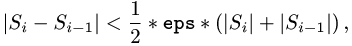
where Si-1 and Si are the observed statistic values for the (i-1) th and i th iteration, respectively. Parameters
SIGMA-REJECTION | SIG-REJThe SIGMA-REJECTION optimization method for fits to 1-D data. Abbreviated equivalents are SIG-REJ and SR. The SIGMA-REJECTION optimization method is based upon the IRAF method SFIT. It iteratively fits data: a best-fit to the data is determined using a "regular" optimization method (e.g. LEVENBERG-MARQUARDT), then outliers data points are filtered out of the dataset, and the data refit, etc. Iterations cease when there is no change in the filter from one iteration to the next, or when the fit has iterated a user-specified maximum number of times. Parameters
SIMPLEXA simplex optimization method. The SIMPLEX method is a single-shot method which attempts to find the local fit-statistic minimum nearest to the starting point. Its principal advantage is that it can work well with complicated statistic surfaces (more so than LEVENBERG-MARQUARDT), while also working quickly (more so than POWELL). Its principal disadvantages are that it has a tendency to "get stuck" in regions with complicated topology before reaching the local fit-statistic minimum, and that there is no guarantee it will find the global fit-statistic minimum. Its tendency to stick means that the user may be best-served by repeating fits until the best-fit point does not change. A simplex is geometrical form in N-dimensional in parameter space which has N + 1 vertices (e.g., in 3-D it is a tetrahedron). The fit statistic is evaluated for each vertex, and one or more points of the simplex are moved, so that the simplex moves towards the nearest local fit-statistic minimum. When a minimum is reached, the simplex may also contract itself, as an amoeba might; hence, the routine is also sometimes called "amoeba." Convergence is reached when the simplex settles into a minimum and all the vertices are within some value eps of each other. The eps parameter controls when the optimization will cease; for SIMPLEX, this will occur when 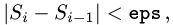
where Si-1 and Si are the observed statistic values for the (i-1) th and i th iteration, respectively. Parameters
SIMUL-ANN-1A simulated annealing search, with one parameter varied at each step. The SIMUL-ANN-1 method is a simulated annealing method. Such a method is said to be useful when a desired global minimum is among many other local minima. It has been derived via an analogy to how metals cool and anneal; as the liquid metal is cooled slowly, the atoms are able to settle into their minimum energy state, i.e. form a crystal. In simulated annealing, the function to be optimized is held to be the analog of energy, and the system slowly "cooled." At each temperature tried, the parameters are randomly varied; when there is no further improvement, the temperature is lowered, and again the parameters are varied some number of times. With sufficiently slow cooling, and sufficient random tries, the algorithm "freezes" near the global minimum. (At each randomization, only one parameter is varied.) This is quite different from the other techniques implemented here, which can be said to head downhill, fast, for a nearby minimum. The great advantage of simulated annealing is that it sometimes goes uphill, thus escaping undesirable local minima the other techniques tend to get stuck in. The great disadvantage, of course, is that it is a slow technique. A simple view of simulated annealing is that a new guess at the location of the minimum of the objective function is acceptable if it causes the value of the function to decrease, and also with probability ![P = exp[-(Delta)f/T]](simul-ann-1_eq1.gif)
where Δf is the increase in the value of the objective function, and T is a "temperature." After a large number of random points in parameter space have been sampled, and no improvement in the minimum value of the objective function has occurred, the temperature is decreased (increasing the probability penalty for positive Δf, and the process is repeated. The expectation is that with a sufficient number of sampled points at each temperature, and a sufficiently slow "cooling" of the system, the result will "freeze out" at the true minimum. The analogy is supposed to be with a cooling gas, where the Boltzmann statistics of molecular motions causes the molecules of the gas to explore both the minimum energy state and adjacent energy states at any one temperature, and then freeze in a crystalline state of minimum energy as the temperature approaches zero. SIMUL-ANN-1 starts with a temperature which is about twice the initial value of the objective function, and reduces it slowly towards zero, changing a single parameter value at each randomization. Parameter tchn is a multiplying factor for the temperature variable between cooling steps. Its default value of 0.98 means that a large number of cooling steps is needed to reduce the temperature sufficiently that the function "freezes out," but fast cooling is not recommended (as it inhibits the ergodic occupation of the search space). Parameter nloop specifies the maximum number of temperature values to try, but may be overridden if the code finds that the solution has "frozen out" early. Finally, parameter nsamp specifies the number of movements at each temperature, i.e. the number of random changes to the parameter values that will be tried. SIMUL-ANN-1 tends to be slow, but is a possible way of making significant progress in traveling-salesman type problems. One of its strengths is that even if it doesn't find the absolutely best solution, it often converges to a solution that is close (in the Δf sense) to the true minimum solution. Somewhat better results are often obtained by SIMUL-POW-1 and SIMUL-POW-2, where the simulated annealing method is combined with the Powell method. Parameters
SIMUL-ANN-2A simulated annealing search, with all parameters varied at each step. The SIMUL-ANN-2 method is a simulated annealing method, analogous to SIMUL-ANN-1 in every way except that at each randomization, all the parameters are varied, not just one. Note that the default temperature cycle change factor, and the number of temperature cycles, correspond to more and faster changes of temperature than SIMUL-ANN-1. This is because of the increased mobility within parameter space, since all values are changed with each randomization. Parameters
SIMUL-POW-1A combination of SIMUL-ANN-1 with POWELL. This method packages together SIMUL-ANN-1 and the POWELL routine; at the end of each of the cooling sequences, or annealing cycles, the POWELL method is invoked. Probably one of the best choices where one "best" answer is to be found, but at the expense of a lot of computer time. Note that the parameters of SIMUL-POW-1 are those of SIMUL-POW-1 itself (which have the same meaning as in routine SIMUL-ANN-1), plus those of POWELL. All of the SIMUL-POW-1 parameters, with the exception of nanne, are explained under SIMUL-ANN-1. Parameter nanne specifies the number of annealing cycles to be used; successive anneal cycles start from cooler temperatures and have slower cooling. The pattern of anneals that has been chosen (the "annealing history") is not magic in any way. A different annealing history may be better for any particular objective function, but the pattern chosen seems to serve well. Parameters
SIMUL-POW-2A combination of SIMUL-ANN-2 with POWELL. This method packages together SIMUL-ANN-2 and the POWELL routine; at the end of each of the cooling sequences, or annealing cycles, the POWELL method is invoked. The rate of cooling in each anneal loop may be much faster than in simulated annealing alone. Probably one of the best choices where one "best" answer is to be found, but at the expense of a lot of computer time.
Note that the parameters of SIMUL-POW-2 are those of
SIMUL-POW-2 itself (which have the same meaning as in
routine SIMUL-ANN-2), plus those of All of the SIMUL-POW-2 parameters, with the exception of nanne, are explained under SIMUL-ANN-2. Parameter nanne specifies the number of annealing cycles to be used; successive anneal cycles start from cooler temperatures and have slower cooling. The pattern of anneals that has been chosen (the "annealing history") is not magic in any way. A different annealing history may be better for any particular objective function, but the pattern chosen seems to serve well. Parameters
USERMETHODA user-defined method. It is possible for the user to create and implement his or her own model, own optimization method, and own statistic function within Sherpa. The User Models, Statistics, and Methods Within Sherpa chapter of the Sherpa Reference Manual has more information on this topic. The tarfile sherpa_user.tar.gz contains the files needed to define the usermethod, e.g Makefiles and Implementation files, plus example files, and it is available from the Sherpa threads page: Data for Sherpa Threads. |
|
The Chandra X-Ray
Center (CXC) is operated for NASA by the Smithsonian Astrophysical Observatory. 60 Garden Street, Cambridge, MA 02138 USA. Email: cxcweb@head.cfa.harvard.edu Smithsonian Institution, Copyright © 1998-2004. All rights reserved. |
 to a
set of observed data, where
to a
set of observed data, where  denotes the model parameters. An optimization
method is one that is used to determine the vector of model
parameter values,
denotes the model parameters. An optimization
method is one that is used to determine the vector of model
parameter values,  , for which the chosen fit statistic is minimized.