Why is there data being plotted or fit outside the energy range I noticed? 

In the following example, we notice energies in the 0.5 to 8.0 keV range, but when the we plot the data, there is a data point above 10 keV. Why?

sherpa> load_pha("9774.pi")
read ARF file 9774.arf
read RMF file 9774.rmf
read background file 9774_bg.pi

sherpa> group_counts(20)
sherpa> notice(0.5, 8.0)
sherpa> plot_data(xlog=True)

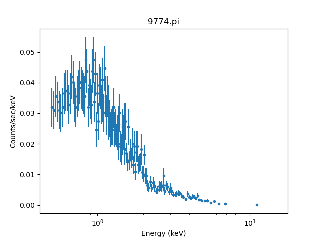
The answer is because the data have been group'ed.

It is important to recognize that there are two distinct spectral axes: energy (usually keV) and detector channel (PI). When you group() your data, this is applied to the data on the detector channel grid. When you notice() an energy range, this is applied to the energy grid the model is evaluated over. The RMF provides the mapping between two grids.

The model is only ever evaluated on the energy grid within the notice'ed energy range. The fit() is only done over the notice()'d energy range.

What is being plotted are the group'ed data. More specifically, the plot shows the middle of each group. As is often the case, in this example the final (right most) group has some channels that correspond energies inside the noticed energy range as well as some channels that correspond to energies outside the noticed energy range. Since the last group includes some channels that are included in the fit, the group -- the entire group -- is shown on the plot.

You can inspect the group boundaries by looking at the data's grouping flags together with the nominal energy-to-channel relation contained in the RMF files "EBOUNDS" extension.

More information

A full discussion of spectral file formats and conventions is beyond the scope of this FAQ. Interested readers can review the documents "The OGIP Spectral File Format" and "The Calibration Requirements for Spectral Analysis"

Sherpa stores the grouping information for a dataset in the arrays: grouping and quality. Groups are encoded as a sequence of values: 1 (start of a new group), -1 (continuation of the group), and 0 (ungrouped). We can use this to get the channel that corresponds to the beginning of each group.

sherpa> mydata = get_data()
sherpa> start_of_groups = np.where(mydata.grouping == 1)

To map channel to energy we can then use the EBOUNDS information from the RMF (the RMF was automatically loaded with the data), and then access the last 5 bins:

sherpa> myrmf = get_rmf()
sherpa> groups_in_keV = myrmf.e_min[start_of_groups]
sherpa> print(groups_in_keV[-5:])
[5.35820007 5.73780012 5.95679998 6.55539989 7.21239996]

From this we see that the final plotted group is the one that starts at a channel that corresponds to 7.2keV Since users may notice different energy ranges during their analysis session, the notice command does not change the grouping flags of the dataset.

Therefore, even though there is a data point above 10 keV, it only contains data from the group with channels less than 8 keV and the model itself is only evaluated up to 8 keV.

Users should be aware that this is also happening with the first group that is being plotted, which we expect to start at 0.5 keV:

sherpa> print(groups_in_kev[(groups_in_kev > 0.47) & (groups_in_kev < 0.53)])
[0.48179999 0.4964     0.51099998 0.52560002]

The first group extends from 0.496 to 0.511 keV. It is just that often the groups at lower energies are smaller so it is more difficult to visually identify this behavior. The same discussion above applies to this end of the spectrum.

The "standard" technique to work around this is to "tab stops" to indicate what ranges of the data you do not want grouped. The aim is to start with an un-grouped and un-filtered dataset, apply the range filter (so it is applied to the native resolution of the data), and then use this filter as a mask in the group_counts call (or other grouping routine). The tricky thing is that the tabStops argument requires the inverse of the data mask, hence the use of NumPy's ~ function to invert the mask:

sherpa> ungroup()
sherpa> notice() 

After ensuring we have no filter or grouping applied, we can identify those channels in the range we are interested with via:

sherpa> notice(0.5, 8.0)
sherpa> mask = get_data().mask

This can then be used in the group_counts call, noting the all-important ~:

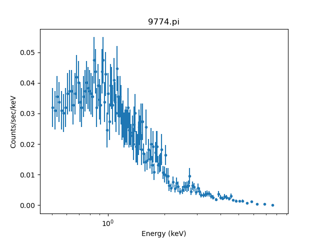
sherpa> group_counts(20, tabStops=~mask)

The result of this is:

sherpa> plot_data(xlog=True)

Incomplete bins

It is highly likely that this scheme - namely using the tabStops argument - will lead to partially-filled bins. In this case it is the last bin (which has a quality value of 2 and not 0):

sherpa> d = get_data()
sherpa> firstChan = d.grouping == 1
sherpa> print(d.quality[firstChan])
[0. 0. 0. 0. 0. 0. 0. 0. 0. 0. 0. 0. 0. 0. 0. 0. 0. 0. 0. 0. 0. 0. 0. 0.
 0. 0. 0. 0. 0. 0. 0. 0. 0. 0. 0. 0. 0. 0. 0. 0. 0. 0. 0. 0. 0. 0. 0. 0.
 0. 0. 0. 0. 0. 0. 0. 0. 0. 0. 0. 0. 0. 0. 0. 0. 0. 0. 0. 0. 0. 0. 0. 0.
 0. 0. 0. 0. 0. 0. 0. 0. 0. 0. 0. 0. 0. 0. 0. 0. 0. 0. 0. 0. 0. 0. 0. 0.
 0. 0. 0. 0. 0. 0. 0. 0. 0. 0. 0. 0. 0. 0. 0. 0. 0. 0. 0. 0. 0. 0. 0. 0.
 0. 0. 0. 0. 0. 0. 0. 0. 0. 0. 0. 0. 0. 0. 2.]

sherpa> print(get_filter())
0.503699988127:7.606600046158
sherpa> print(f"Number of selected bins: {d.mask.sum()}")
Number of selected bins: 135

The ignore_bad function will remove these partial bins, but it resets the filters on the dataset:

sherpa> ignore_bad()
WARNING: filtering grouped data with quality flags, previous filters deleted
sherpa> notice(0.5, 8)
sherpa> print(get_filter())
0.503699988127:6.883899927139
sherpa> print(f"Number of selected bins: {d.mask.sum()}")
Number of selected bins: 134

If we were to plot the data we would see that the last bin in the previous plot would now be removed.