

Astronomers analyze spectral energy distributions (SEDs) by fitting them with models over a wide range in wavelength, from gamma rays to radio waves. The resulting best-fit values for the SED model parameters, and associated confidence limits, are physically meaningful quantities. The Iris SED analysis tool allows for robust modeling and fitting of SED data through association with Sherpa, an extensible, Python-based, multi-waveband modeling and fitting application for astronomers.
Learn how to fit models to SED data in Iris with custom model expressions, including preset and/or your own model components; how to set initial model parameter values and ranges, and choose an appropriate fit statistic and method; as well as calculate errors on best-fit model parameters.
Last Update: Feb 22 2017 - updated for Iris 3.0.
After one or more SED data segments and/or photometric points have been read into Iris, and data display preferences set, the data may be fit with a customized model using the Fitting Tool. Clicking the Fitting Tool icon ![]() opens a new window in which individual model components may be combined to define a custom model expression, and where initial model parameter values and the spectral fitting ranges are set.
opens a new window in which individual model components may be combined to define a custom model expression, and where initial model parameter values and the spectral fitting ranges are set.
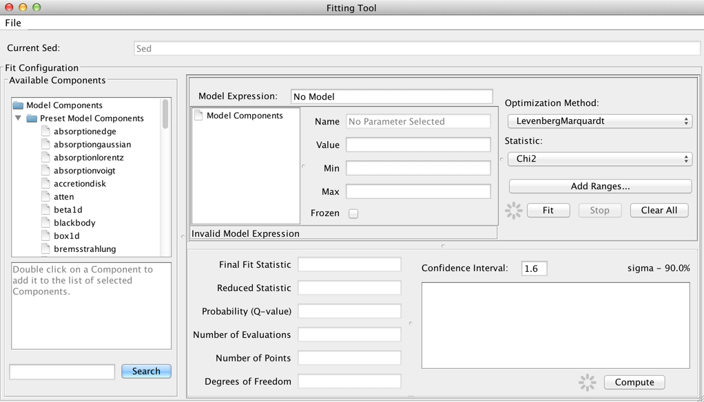
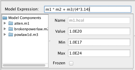
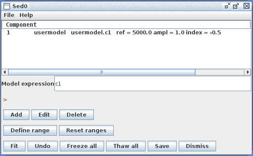
The Model Components section of the fitting window lists the model components used to construct the full model expression for fitting; these components can then be arbitrarily combined to form the full model expression, in the Model Expression field. Components are referenced by a model identifier “m#”, where the number increases for each new component added to the Model Components list.
Model amplitudes are in units of photon flux density by default, and model spectral coordinates are in Angstroms. Currently, the default fit results units cannot be changed.
| [Back to top] |
Model expressions are defined by combining model components together in the Model Expression field at the top of the Fitting Tool frame.
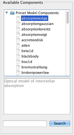
The list of available models is shown on the left-most panel of the Fitting Tool. Double-clicking a model will add it to the list of model components. By default, components are linearly combined in the Model Expression field when a model is added.
Iris is distributed with a list of preset optical and X-ray Sherpa models. A brief description of the model is displayed below the list when the users highlights a model name. More in depth-descriptions of the Sherpa models are discussed in Iris Models.
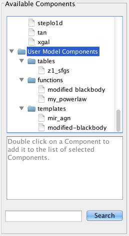
There is also the option to choose a custom template, template library, or Python user model which you may have imported into the session via the Iris “Custom Models Manager” tool (see “Importing Custom Models” below to learn how to import custom models into Iris).
Components may be added or multiplied together arbitrarily, which allows the modeling of emission and/or absorption features as well as the ability to apply a more complex model to the continuum itself.
For a simple model, such as an expression containing one model component, defining the model is trivial: write the component ID of the model component, e.g., “m1”, in the Model Expression field. For a composite model, add, subtract, multiply, and/or divide the model components as needed to model your SED, such as “m1*m2 + m3/(4*3.14)”. Note that numbers may be used directly in the model expression as well.
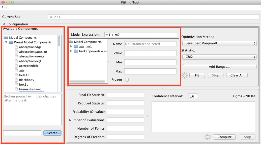
Consider the example of fitting an absorbed broken power-law model to an SED of object 3C 273. You would select and add “atten” and “brokenpowerlaw” from the list of preset Iris models, which adds both models to the Model Components section of the fitting window.
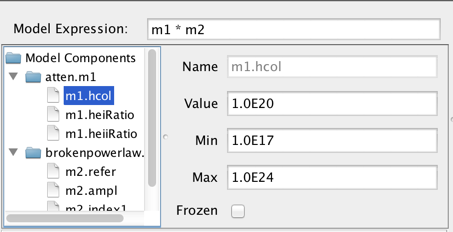
Then, you would define the model expression as the product of the two components: “m1*m2”.
Each component in the Model Components list may be expanded to show each component’s model parameters. From here, the user can select the model parameters and set the initial parameter values and ranges by editing the fields shown to the right of the Components list.
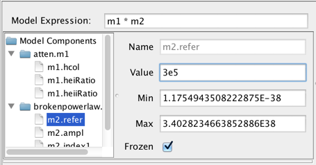
The parameter minimum and maximum values may be specified. The “Frozen” checkbox is for specifying whether or not to freeze that parameter during the fit; if unchecked, the parameter will be allowed to vary.
Note: flux and spectral parameter values must be in units of photons/s/cm2/Angstrom and Angstroms, respectively.
The initial model parameter values are where Sherpa starts the fit in parameter space; the parameter ranges are the bounds of parameter space. It is not possible to fit using parameter values outside the specified parameter ranges.
| [Back to top] |
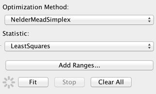
The next step in the preparation for fitting involves choosing a fit statistic and optimization method appropriate for your analysis. These methods are listed below with brief descriptions. For more detailed descriptions, please refer to the Statistics and Optimization pages of the Sherpa website.
| Optimization Method | Description |
|---|---|
| Levenberg-Marquardt | a method to find the best-fit model parameter values, by finding the local minimum in parameter space; the functions to be minimized are nonlinear least-squares functions, of the model parameters. |
| Nelder-Mead | a method to find the best-fit model parameter,values, by finding the local minimum in parameter space; a direct,search method is used to continually move "downhill" in parameter,space, until settling in a local minimum. |
| Monte Carlo | a method using the differential evolution,algorithm, to find a global minimum in parameter space; the search,is seeded with randomly selected starting points, and can continue,the search for the true minimum where the other methods could get,stuck in local minima that do not represent the actual best fit.,(Most useful for complex models and fits that could explore,complicated regions of parameter space.) |
| Statistic | Description |
|---|---|
| Chi2 | |
| Chi2DataVar | Chi-squared statistic with variance computed from the data. If measured errors are provided, the variance is taken from these errors; else, the variance is computed from the y-values of the data points. |
| Chi2Gehrels | Chi-squared statistic, where the variance is computed with a function from Gehrels et al. Suitable for low counts data (e.g., X-ray data) to correct for bias in using chi-squared. |
| Chi2ModelVariance | Chi-squared statistic, where the variance is computed from the model values instead of data. |
| Chi2ConstantVariance | Chi-squared statistic, where the variance is set to be a constant value. That constant is the average of the y-values of the data points. |
| Chi2XspecVariance | Chi-squared statistic, where the variance is computed as the X-ray spectral fitting program XSPEC would compute the variance (i.e., where the variance would be less than one, reset it to one). More suitable for low counts data (e.g., X-ray data). |
| CStat | A maximum likelihood function similar to Cash, but with a chi-squared-like probability distribution. More suitable for counts data than for fluxes. |
| Cash | A maximum likelihood function based on Poisson statistics. More suitable for counts data than for fluxes. |
| LeastSquares | Sum of the squares of the differences between, data and model values. |
The default fitting method and statistic are “NelderMeadSimplex” and “LeastSquares”, respectively, which represent good choices for a robust, quick, initial fit of a relatively simple model to a data set covering potentially many orders of magnitude in flux and/or wavelength. The fit can also be done with a chi-squared statistic or with a maximum likelihood statistic useful for data with low number counts. The optimization method can be changed to “Levenberg-Marquardt” or “Monte Carlo”, but note that switching the method is less important than switching the statistic, e.g., from least-squares to chi-squared.
Nelder-Mead is the optimal fitting method to start with because it does not depend on taking derivatives of the model function. As for the fit statistic, least-squares is preferred because it does not use measured errors and thus essentially weights all data points equally (it seeks to minimize the sum of the squares of the differences between data and model values, without taking errors into account). Chi-squared fitting, in contrast, can be decidedly biased towards the data points with the lowest fluxes and smallest measured error bars. In other words, when there are data points with measured errors that are orders of magnitude smaller than the error bars on most of the data points, then these points become the biggest contributors to the chi-squared value.
In subsequent fits - e.g., after selecting a different data range to fit, adding in new model components as needed, and so on - the statistic can be switched to a chi-squared option to use measured errors (preferably “Chi2” or “Chi2Datavar” for high counts (>5) data points; “Chi2Gehrels” or “Chi2XspecVariance” for low counts data). If measured errors are provided, the variance is taken directly from the errors provided with the data.
Note: When one or multiple SED segments is fit in Iris, any data points with associated zero-value errors are ignored in the fit. This design choice is intended as a safeguard against yielding potentially misleading fit results in the analysis of your SED data. Iris interprets a zero-value error not to mean that the uncertainty on the associated data value is actually zero, but that a measure of the uncertainty is not available for that particular photometric point.
| [Back to top] |
Before initiating a fit of the defined model to a SED, the specific subset of the SED data to be included in the fit (if not the entire SED) may be specified using the “Add Range..” option in the main fitting window. This opens a Fitting Ranges manager window in which a user defines the fitting range(s) for the fit.
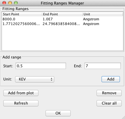
A fitting range may be defined by two ways:
Fitting ranges may be removed by highlighting the ranges and clicking “Remove”; all ranges can be removed with the “Clear all” button.
The fitting ranges appear on the Visualizer as a blue horizontal line.
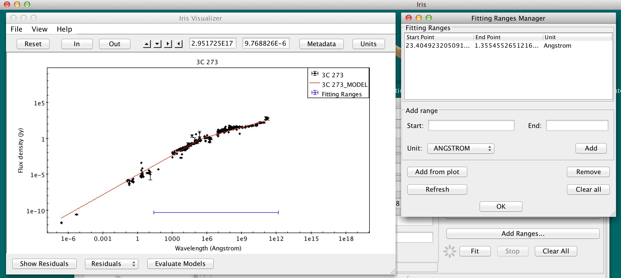
Defining multiple fitting ranges is useful for masking out spectral features when fitting the continuum of a spectrum.
| [Back to top] |
Having built a model expression and set initial parameter values, chosen an appropriate fit statistic and optimization method for your analysis, and defining the range of data to be fit, you are ready to initiate the fitting process.
Click “Fit” in the Fitting Tool window to start the fit. When the fit is complete, a red model curve appears overplotted on the SED data in the Visualizer (Note that the red line may be plotted beyond the specified data range to be fit; this extraneous portion of the fitted model may be ignored).
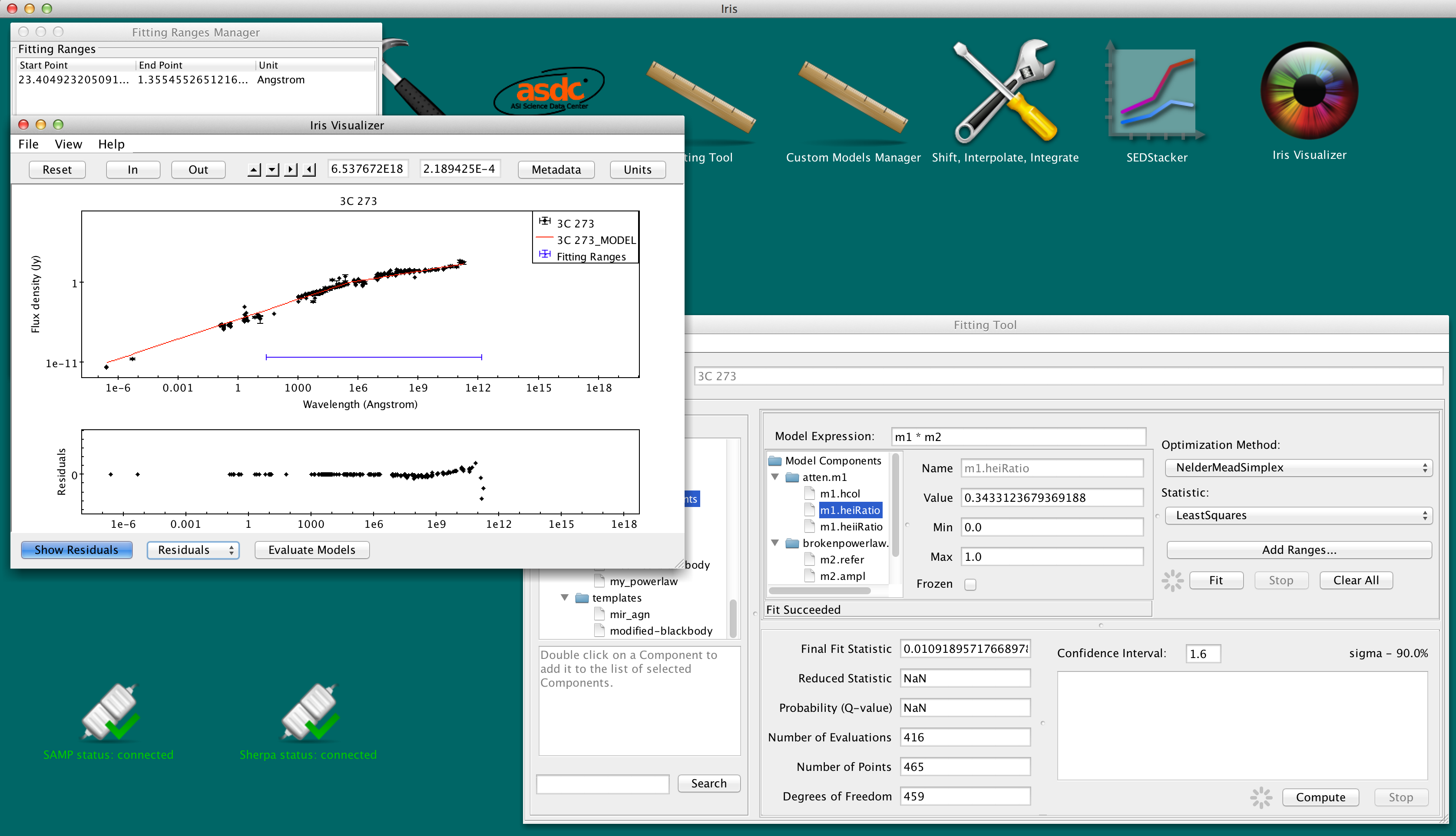
When the fit has finished, the model parameter values will appear updated in the Model Components fields, and fit statistics will be displayed in the bottom panel. The fit results include
*The Q-value and reduced statistic are unavailable when fitting with the least-squares or Cash, as they cannot be computed for those statistics.
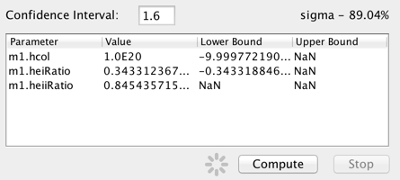
When fitting with one of the chi-squared statisics, or the chi-squared-like Cstat statistic, the confidence limits of the fitted model parameter values may be calculated.
Enter the the confidence interval in terms of sigma and click “Compute” to calculate the upper and lower confidence limits for the on the best-fit model parameters. For example, entering “1.6” in the “sigma” field will return the 90% confidence limits on the model parameter values. The limits are calculated using the statistic and method chosen for the fit.
If the statistic is left at the default “leastsq”, Iris will issue an error stating that least-squares cannot be used with the confidence limit function (this is because the only way calculate to confidence limits is to know the probability distribution for the fit statistic, which is known for the chi-squared and chi-squared-lke cstat statistic, but not least squares).
Also of note is that blank or “NaN” values are returned in the confidence results when a parameter bound is found to lie outside the hard limit boundary for a model parameter (which ought not to be changed by the user, so there is not an option to do so in Iris). This could result from an issue with the signal-to-noise of the data, the applicability of the model to the data, systematic errors in the data, among others things. A parameter hard limit represents either a hard physical limit (e.g., temperature is not allowed to go below zero), a mathematical limit (e.g., prevent a number from going to zero or below, when the log of that number will be taken), or the limit of what a float or double can hold (the fit should not be driven above or below the maximum or minimum values a variable can hold).
You can iterate through the fitting process in Iris as many times as necessary - adding or deleting models from the model expression; changing parameter values or ranges; including or excluding new points from the SED - until you find a satisfactory model that best describes your SED data.
| [Back to top] |
Once a spectral model is satisfactorily fitted, the fitted model parameters can be saved to a local file by making an appropriate selection in the File menu of the fitting window.
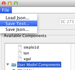
Selecting File -> Save Text… saves the model and fit results to file in a human-readable text format. Example output is shown below:
$ more 3c273_atten_bpl_active_comps.txt

Iris Fitting Tool - Fit Summary
SED ID: Sed (Segments: 1)

Model Expression: m3 * m4
Components:
        brokenpowerlaw.m3
                                  m3.refer =  3.00000E+05 Frozen
                                   m3.ampl =  2.50378E-03
                                 m3.index1 = -5.21571E-01
                                 m3.index2 = -4.78847E-01
        atten.m4
                                   m4.hcol =  1.00000E+20 Frozen
                               m4.heiRatio =  3.59464E-01 Frozen
                              m4.heiiRatio =  9.69470E-01 Frozen

Fit Results:
                       Final Fit Statistic =  3.26931E+07
                         Reduced Statistic =  8.69497E+04
                     Probability (Q-value) =  0.00000E+00
                        Degrees of Freedom = 376
                               Data Points = 379
                      Function Evaluations = 511

                                 Optimizer = NelderMeadSimplex
                 Statistic (Cost function) = Chi2

Confidence Limits at 1.60 sigma (89.04%):
                 m3.ampl: (-1.94416E-07,  1.94620E-07)
               m3.index1: (-4.21899E-05,  4.22327E-05)
               m3.index2: (-2.62248E-04,  2.61584E-04)
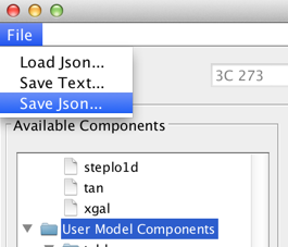
Selecting File -> Save Json…, instead, saves the model to a file in Json format that can be read back by the tool in a future data analysis session.
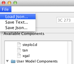
This customized Iris fitting session may be restored by selecting the File->Load Json… menu option within the Iris fitting window.
Restored models may be evaluated or refit to other SEDs.
To evaluate a model on an SED (without refitting), open the Fitting Tool, load the Json file into the fitting session, then open the Visualizer and click “Evaluate” (at the bottom of the plot window). This will overplot the model on the data, and recalculate the fit statistics.
| [Back to top] |
As it may be necessary to fit data with a model that does not come pre-packaged with Iris, the Custom Model Manager interface is available for configuring and importing your custom tables, template libraries, or Python function user models into the Iris fitting session.
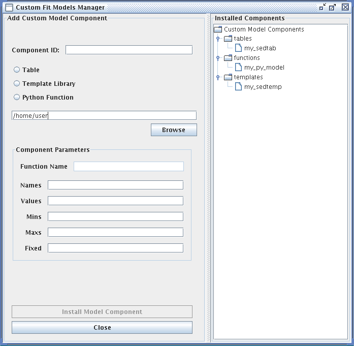
Custom models must be defined in a file. To add a custom model, you must define the path to the model file, the model type – table, template library, or Python function – the model ID, and the model parameters. After installing the model, it can be selected from the list of Model Components and added to a model expression for fitting, under User Model Components -> tables/functions/templates -> “your model string ID”.
The fields of the Custom Model Manager window are described below:
Component ID - an arbitrary string to identify the custom model for storage in Iris
“Table” radio button - identifies the custom model as a table read from file. The data contained in custom table models must have the same units that Iris uses internally for modeling and fitting. The x-axis units must be in Angstroms, and the y-axis units must be in photons/s/cm^2^/Angstrom.
“Template Library” radio button - identifies the custom model as a set of templates read from files. The data contained in custom template models must have the same units that Iris uses internally for modeling and fitting. The x-axis units must be in Angstroms, and the y-axis units must be in photons/s/cm^2^/Angstrom.
“Python Function” radio button - identifies the custom model as a function that will be imported from Python
In the text box beneath the radio buttons, type in the full path to the file containing the custom model, e.g., “<your_path_to_file>/mypowlaw.py” for the “Python Function” option.
Component Parameters -> Function Name - the name of the Python function to be added as a user model, used only for the Python Function option
Component Parameters -> Names - names of the model parameters, separated by commas
Component Parameters -> Values - the initial parameter values corresponding the parameter names listed above, separated by commas
Component Parameters -> Mins - the minimum allowed values, separated by commas.
Component Parameters -> Maxs - the maximum allowed values, separated by commas.
Component Parameters -> Fixed - Boolean values, separated by commas, indicating whether parameters are fixed at the initial value during the fit (True = fixed at starting value, False = allowed to vary during the fit.)
Install Model Component - install the model as a custom model in Iris. The next time the Fitting Tool is opened, the model can be selected from the menu of custom model components, under Add -> Custom Model Components -> functions -> “your model component ID”.
| [Back to top] |
Iris supports ASCII-format table model files consisting of two separated columns of numbers, the X (spectral coordinate) and Y (flux) data values. When the table model is “calculated” during a fit, it returns the array of Y values multiplied by a single parameter for the model, amplitude. The amplitude parameter can be varied during the fit (i.e., a scale factor applied to the tabular data).
Example entries in the Custom Model Manger window are shown in the image below for a custom power-law table model.
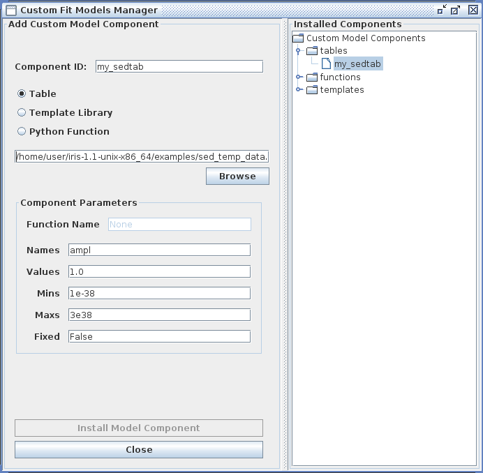
The example table model file “sed_temp_data.dat” - which can be found in the “examples” directory of your Iris installation - is shown below, where the X column contains wavelength values in units of Angstroms, and the Y column is flux density in units of photons/s/cm^2^/Angstrom (the internal units used for fitting in Iris are always photons/s/cm^2^Angstrom against Angstroms).
% more <basedir>/miniconda/iris/opt/iris/examples/sed_temp_data.dat

   4.8588736e-06   8.4482890e-03
   1.7739201e-01   4.0325498e-03
   2.0675345e-01   9.2701427e-03
   3.2201128e-01   6.9831383e-03
   3.5436466e-01   9.1989617e-03
   4.1350690e-01   2.8576857e-03
   2.0675345e+00   4.1752139e-03
   2.3793056e+00   6.1398901e-03
   2.4776240e+00   1.1573206e-02
   3.1002327e+00   2.4582868e-03
   6.5314270e+00   3.7663007e-03
   9.2243846e+00   5.8898001e-03
   9.9269040e+00   2.2043961e-03
   1.2388120e+01   1.3400554e-03
   6.1940599e+01   1.1914311e-03
   9.9930833e+02   1.8273482e-02
   1.0302148e+03   3.5890026e-03
        .               .
        .               .
        .               .
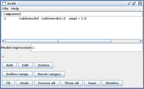
Clicking “Install Model Component” installs the model as a custom model in Iris. The next time the Fitting Tool is opened, the model can be selected from the menu of custom model components, under User Model Components -> tables -> my_sedtab.
| [Back to top] |
Iris also supports template model libraries so that you may compare a source data spectrum against a set of template models, in order to find the single template model which best matches the source data. During the fit, the data are compared to each template, to determine which template is the closest match to the data. The parameters associated with that template are returned as the best-fit parameters.
A collection of template models may be read into Iris by entering into the Custom Model Manager window the name of a single ASCII index file which lists the file contents of a directory full of template model files, in addition to the model parameter values associated with each template file. The various model files should also be in ASCII format, and contain separated columns of X and Y coordinates, where the X column lists the wavelength in Angstroms, and the Y column is the flux density in photons/s/cm^2^/Angstrom.
The Iris Custom Model Manager window would appear as shown below when loading a template model library, where the template model index filename is entered into the “Add Custom Model Component” section, and the template model parameter information is entered into the “Component Parameters” section. In the “Component Parameters -> Names” field, the parameter names should match the names listed as parameters in the template index file.
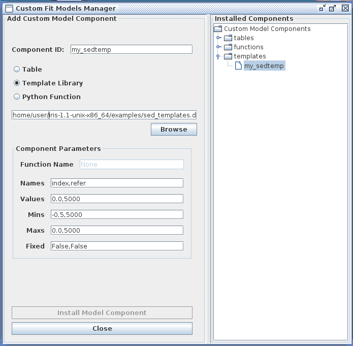
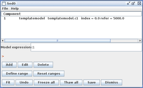
Clicking “Install Model Component” installs the model as a custom model in Iris. The next time the Fitting Tool is opened, the model can be selected from the menu of custom model components, under Add -> Custom Model Components -> tables -> my_sedtemp.
Consider the example template model shown below, a representative of a set of power-law models, where there is a separate model file for each combination of model parameter values (power-law reference point and photon index, in this example).
$ ls <basedir>/miniconda/envs/iris/opt/iris/examples/sed_temp_index*.dat

<basedir>/miniconda/envs/iris/opt/iris/examples/sed_temp_index-0.00.dat
<basedir>/miniconda/envs/iris/opt/iris/examples/sed_temp_index-0.10.dat
<basedir>/miniconda/envs/iris/opt/iris/examples/sed_temp_index-0.25.dat
<basedir>/miniconda/envs/iris/opt/iris/examples/sed_temp_index-0.35.dat
<basedir>/miniconda/envs/iris/opt/iris/examples/sed_temp_index-0.50.dat


$ ls <basedir>/miniconda/envs/iris/opt/iris/examples/sed_temp_index-0.10.dat

4.8588736000000e-06 1.2188068071007e-03
1.7739201000000e-01 4.2628006741162e-04
2.0675345000000e-01 4.1980069644345e-04
3.2201128000000e-01 4.0160704511216e-04
3.5436466000000e-01 3.9778040979499e-04
4.1350690000000e-01 3.9168789965186e-04
.
.
.
Each of the ASCII-format template files listed above contains columns of wavelength in Angstroms and flux density in photons/s/cm^2^/Angstrom (the internal units for fitting in Iris are always photons/s/cm^2^/Angstrom against Angstroms), defining the predicted power-law spectra emitted by an X-ray source.
The template model index file which is entered into the Custom Model Manager window should contain a table with one line per template data file, with three groups of columns in the following order:
The MODELFLAG column, which separates the parameter list from the filenames/model arrays, marks lines which are to be used or not: MODELFLAG = 1 - use the file; MODELFLAG = 0 - do not use the file (note that the MODELFLAG column in this file is not a model parameter)
The FILENAME column which points to the data file for that instance, including the full directory path to the file.
Iris reads the index file in order to set up the template model with the parameters specified in the first line, and the arrays from the columns given by the data files.
An example index file appears below, with model flags (all having value 1) and filenames listed in the two right-most columns, and the power-law photon index and reference point model parameters listed from the left. The combination of the two parameter values sets the spectral shape of the model.
$  more <basedir>/miniconda/envs/iris/opt/iris/examples/sed_templates.dat

# IDX REFER MODELFLAG FILENAME
0.0     5000  1   <basedir>/miniconda/envs/iris/opt/iris/examples/sed_temp_index-0.00.dat
-0.10   5000  1   <basedir>/miniconda/envs/iris/opt/iris/examples/sed_temp_index-0.10.dat
-0.25   5000  1   <basedir>/miniconda/envs/iris/opt/iris/examples/sed_temp_index-0.25.dat
-0.35   5000  1   <basedir>/miniconda/envs/iris/opt/iris/examples/sed_temp_index-0.35.dat
-0.50   5000  1   <basedir>/miniconda/envs/iris/opt/iris/examples/sed_temp_index-0.50.dat
Linear interpolation is used by the template model to match the data grid to the model grid - which must match before the fit statistics can be calculated for fitting. Instead of a simple grid-search method, K-nearest neighbor interpolation is used to evaluate the best-fit parameter values, with k=2 and order=2. The parameter values returned are a weighted interpolation between two best-fit templates.
| [Back to top] |
You also have the option of importing into Iris a custom model function which you have defined and written in the Python scripting language. The name of the Python file in which it is saved is entered into the Iris Custom Model Manager interface with the “Python function” option selected, as shown below for an example using a power-law function. Note that the Component Parameters -> Function Name field becomes active when this option is selected.
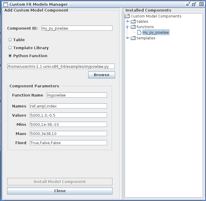
The contents of an example Python user model file is shown below, where a power-law model function named “mypowlaw” is defined:
$ more powlaw.py

import numpy

def mypowlaw(p, x):
    arg = x / p[0]
    arg = p[1] * numpy.power(arg, p[2])

    return arg
The ‘p’ and ‘x’ function arguments represent the arrays of parameter values and x-values, respectively. For this example, the model parameters entered into the Component Parameters section of the Custom Model Manager window are the normalization reference point, amplitude, and photon index of the power-law model. The “Function Name” entered into this section must match the Python function name in the file, “mypowlaw”.
Clicking “Install Model Component” installs the model as a custom model in Iris. The next time the Fitting Tool is opened, the model can be selected from the menu of custom model components, under User Model Components -> functions -> my_py_powlaw.
| [Back to top] |
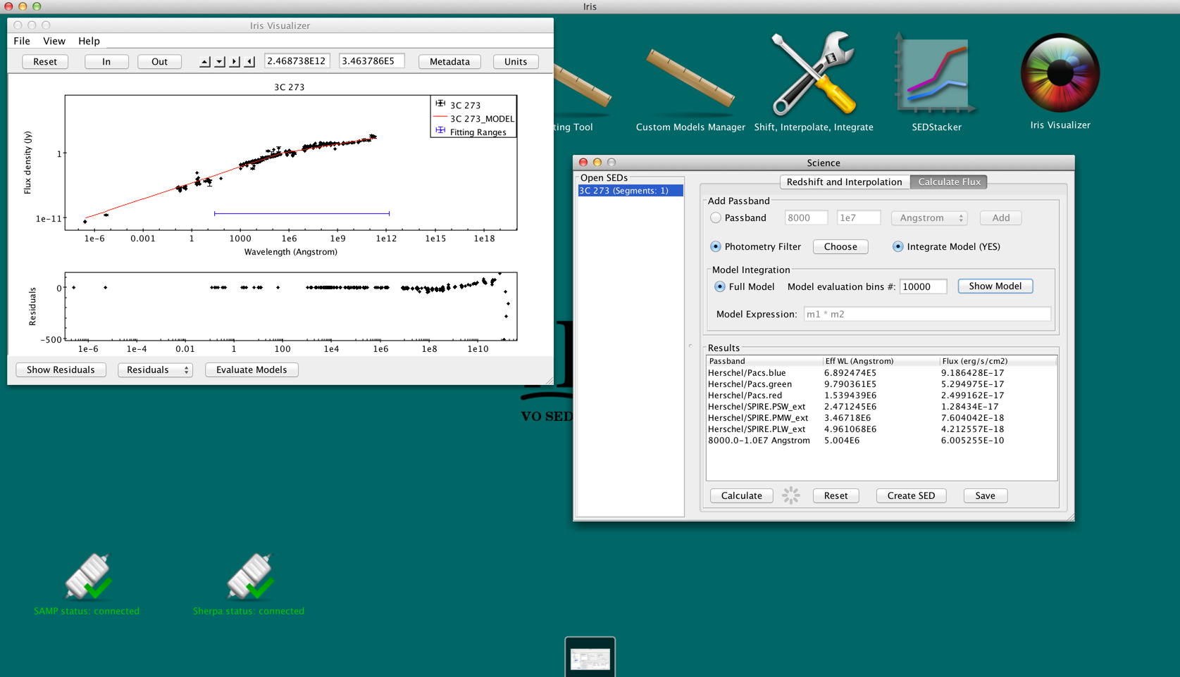
After fitting a SED, you can estimate fluxes through user-defined passbands and photometric filters by integrating under the model components. This is done from the “Calculate Flux” tab in the Science tools, which is opened by clicking the “Shift, Interpolate, Integrate” icon on the desktop. The user may integrate under the full model or an arbitrary combination of the model components. The Fitting Tool must remain open for model integration.
![[Calculate Flux screenshot]](./imgs/integrate_under_model-default.png)
After opening the “Calculate Flux” tab, make sure Model Integration is selected (it should “Integrate Model (YES)”). By default, the full model will be used to evaluate the fluxes. For our fit of 3c273, the model expression is "m1*m2". A quick-look view of the model and the parameter values can be displayed by clicking the “Show Model” button.

You can change the number of spectral bins used to calculate the integral by adjusting the value in the “Model evaluation bin #” box.
By checking-off “Full model,” the user can arbitrarily combine the model components, then integrate the expression in the “Model Expression” field. This means that users can integrate under individual model components. Multiplication and addition of other model components and numeric values are acceptable. For example, the expressions "m2 * 3.678", "m2 + m1", and "m1 + m2 * 1.2" are allowed.
Say we want to estimate the total infrared flux and the flux through the Herschel PACS and SPIRE bands . Going back to the “Calculate Flux” in the Science tool, we add the Hershcel photometry filters (select “Photometry Filter” -> “Choose” and search for “Herschel”) and add a user-defined pass band from 0.8 to 1000 microns (8000 - 1E7 Angstroms). To integrate under the fitted model, we turn “Model Integration” on (YES), and click “Calculate.”
The results can be exported as a new SED with the “Create SED” button, or may be saved to a text file with “Save.” The text file can be loaded back into Iris as an ASCII Table.
NOTE: If the user exits the main Fitting Tool window, the user will no longer be able to integrate under the fitted model, as the models will be lost from closing the fitting session. Iris will ask the user if they really want to leave the fitting session if they try to close the Fitting Tool.
| [Back to top] |
| Date | Changes |
|---|---|
| 09 Aug 2011 | updated for Beta 2.5 |
| 25 Sep 2011 | updated for Iris 1.0 |
| 08 Jun 2012 | updated for Iris 1.1 |
| 02 Jan 2013 | updated for Iris 1.2 |
| 21 Jun 2013 | updated for Iris 2.0 |
| 05 Aug 2013 | updated Iris screenshots |
| 02 Dec 2013 | updated for Iris 2.0.1 |
| 07 May 2015 | updated for Iris 2.1 beta. Users can now integrate under fitted models. Template library model parameter values are interpolated using k-nearest neighbor with k=2 and order=2. Templates, table models, and functions can all be arbitrarily combined in the Model Expression. |
| 01 Jan 2017 | updated for Iris 3.0b2 |
| 22 Feb 2017 | updated for Iris 3.0 |
| [Back to top] |