Next: 12. Advanced wavdetect: Using Up: The Detect Reference Manual Previous: 10. vtpdetect Parameters & Contents
This section highlights some frequently used wavdetect parameters. Similar parameters and their description have been grouped together. Chapter 14 has information on each wavdetect parameter in alphabetical order.
The input file can an event list or an image. CIAO Data Manipulation (DM) syntax may be used in the input file specification, as explained in Chapter 1, Section 1.3.3.
Be careful using images larger than 1024![]() 1024, as a large
amount of computer memory must be available.
1024, as a large
amount of computer memory must be available.
The outfile parameter is used to provide a name for the output file. The kernel parameter controls the output format; the default is for the output file to have the same format as the input file. If autonaming is used (i.e. "outfile=."), then the output file will be named "<infile_root>_src".
The scellfile is the image showing the source cells. These source cells delimit the image pixels that are used to estimate source properties (e.g. count rate). If autonaming is used (i.e. "scellfile=."), then the output file will be named "<infile_root>_scell".
The reconstructed source image filename is given by the imagefile parameter. If autonaming is used (i.e. "imagefile=."), then the output file will be named "<infile_root>_image".
The output file that will contain the default normalized (i.e. flat-fielded) background is specified by the defnbkgfile parameter. During its second stage, wavdetect makes one normalized background estimate from the stack of per-scale normalized backgrounds produced during the first stage. It writes the computed background to this file. If autonaming is used (i.e. "defnbkgfile=."), then the output file will be named "<infile_root>_nbkg".
To obtain true count rates with wavdetect , the output values must be divided by the exposure time. If an exposure map is not provided, a dummy array with all pixel values set to 1 will be used.
The exptime parameter specifies the length of time in seconds over which the field was observed. If set to 0, the value will either be taken from the expfile FITS header or, failing that, estimated by averaging over exposure map pixel values at the center of the field.
The expthresh parameter specifies the minimum relative exposure needed in a pixel in order to analyze it. This parameter should not be less than 0.1 or the accuracy of normalization will be too low. If set close to 1, only very limited regions of the field of view will be considered when source correlation maxima are listed. Typical values are 0.1-0.2.
The scales parameter determines how
many scaled transforms will be computed. wtransform produces a
complete set of outputs for each scale. Small scales tend to
detect small features, and larger scales find larger features.
The units for scales are pixels. The
value of scales is the radius of the Mexican Hat function,
which crosses zero at
![]() radius.
radius.
For the initial run, try the default value "2.0 4.0". If that
test is successful, try again with
scales "1.0 2.0 4.0 8.0 16.0".
For a more extensive run, the user might wish to try the ![]() series: "1.0 1.414 2.0 2.828 4.0 5.657 8.0 11.314
16.0".
series: "1.0 1.414 2.0 2.828 4.0 5.657 8.0 11.314
16.0".
The primary concern regarding this parameter is to match the first
scale size to the point spread function (PSF). Once that is done, the
user must decide how many scaled wavelets to use. To some extent,
choices are based on the computing resources at hand. Reasonable
inputs are a 512![]() 512 array and 5 to 9 scales, where each scale
is a factor of 2 or
512 array and 5 to 9 scales, where each scale
is a factor of 2 or ![]() larger than the preceeding one.
larger than the preceeding one.
In practice, one must not have too many pixels or scale sizes,
otherwise the computational load becomes a problem. Data structures
for a 512![]() 512 image use up 36 MB, while a 2048
512 image use up 36 MB, while a 2048![]() 2048
image requires over 300 MB. Datasets that do not fit in physical
memory will page heavily to disk and processing will progress very
slowly. Scale sizes larger than 32 allocate excessive memory because
it is necessary to pad the image with surrounding zeros.
2048
image requires over 300 MB. Datasets that do not fit in physical
memory will page heavily to disk and processing will progress very
slowly. Scale sizes larger than 32 allocate excessive memory because
it is necessary to pad the image with surrounding zeros.
To deal with resolved sources, several convolutions are performed, each with a successively larger scale version of the wavelet. The resulting "correlation maps" are then examined for regions where the intensity is larger than some threshold, and the final source list is constructed from a comparison of the different scale runs.
The significance threshold for source detection. A good value to use
is the inverse of the total number of pixels in the image, e.g. ![]() 10
10![]() (the default) for a 1024
(the default) for a 1024![]() 1024 field. This is
equivalent to stating that the expected number of false sources per
field is one. If larger arrays are used without decreasing the value
of sigthresh , there will be an
increased probability of detecting false sources. Likewise, if smaller
arrays are used, the user may wish to increase this parameter value.
The sigthresh should not be
smaller than roughly
1024 field. This is
equivalent to stating that the expected number of false sources per
field is one. If larger arrays are used without decreasing the value
of sigthresh , there will be an
increased probability of detecting false sources. Likewise, if smaller
arrays are used, the user may wish to increase this parameter value.
The sigthresh should not be
smaller than roughly ![]() 10
10![]() to
to ![]() 10
10![]() ; at this
value, the accuracy of the computed detection thresholds is unknown.
; at this
value, the accuracy of the computed detection thresholds is unknown.
In addition to the output source list (outfile ), the user may choose to have an ASCII source region file written by specifying a filename in regfile parameter. If autonaming is used (i.e. "regfile=."), then the source regions output file will be named "<infile_root>_reg".
This region file is useful for subsequent input into ds9, particularly to overlay region markers over each detection; see Chapter 1, Section 1.4 for details.
The size of the elliptical source regions in both of the source region files is controlled via the ellsigma parameter. This parameter is a multiplicative factor applied to sigma, the standard deviation of the distribution, to scale the major and minor axes of the ellipses for each source detection. This feature is included so that the graphics overlay may be made more visible; it is does not affect the detections themselves, only the display of the regions.
By default the value for ellsigma is 3, but a larger value is often helpful.
The maximum number of iterations per scale pair for cleaning sources
from the data in order to estimate the background map; the default is
2. Increasing this number will increase the method's source detection
sensitivity, but may not increase it enough to justify the increased
computation time. More iterations are generally needed for large
wavelet scales (e.g. 16 pixels in a Rosat 512![]() 512 PSPC
field). Note that the tool may converge before reaching
maxiter .
512 PSPC
field). Note that the tool may converge before reaching
maxiter .
If the ratio of newly cleansed pixels to the overall number of pixels in the dataset is less than the parameter iterstop when wavdetect constructs a default normalized (i.e. flat-fielded) background (defnbkgfile ), then wavdetect stops iterating and uses the current background estimate as the final background estimate. The background is calculated if there are very few new pixels being cleansed (see bkgsigthresh ).
The iterstop parameter specifies how many iterations the program should go through to calculate the background. A typical value is 0.0001 (the default): stop iterating when one of every thousand pixels has been cleansed. This parameter should not be smaller than one over the number of pixels in the dataset or larger than 1.
A significance for cleaning data from the image to compute the
background map. As it does not effect source detection, this parameter
should be set to a more liberal value than
sigthresh (e.g. 10![]() or
10
or
10![]() , the default), but not smaller than
sigthresh ). This will help
reduce the effect of weak undetectable sources on the background map
calculation. This value should be no larger than 0.05, the usual 5%
(or 95%) statistical criterion for rejecting the null hypothesis,
which is that the pixel in question has data sampled solely from the
background.
, the default), but not smaller than
sigthresh ). This will help
reduce the effect of weak undetectable sources on the background map
calculation. This value should be no larger than 0.05, the usual 5%
(or 95%) statistical criterion for rejecting the null hypothesis,
which is that the pixel in question has data sampled solely from the
background.
If desired, a previously computed background image may be input instead of allowing wavdetect to construct a default normalized background. When using bkginput , enter none for the default normalized background output file (defnbkgfile ).
If bkgerrinput is changed to yes, then the background error data in the second extension of the bkginput file will be used (i.e. "bkginputfilename.fits[2]'').
The bkgtime parameter may specify the LIVETIME value for the provided background.
In wavdetect , PSF, energy, and offset information supplied via these parameters is used to select a source counts image; a source cell is computed using this image, and source properties are estimated using the data within the computed cell. Note that, unlike celldetect , these parameter values have no effect on the detection process. Instead, these parameter values affect reported source properties.
The PSF information used by wavdetect is contained in a Chandra calibration file distributed with CIAO , whose location is given by the value of the psftable parameter; by default this parameter is automatically set to point to the appropriate Chandra calibration PSF file.
The selection of a particular PSF size is governed by the energy band parameter eband , in keV (since the Chandra PSF is a function of energy). By default the energy band is set to 1.4967 keV, but the user may wish to adjust this value.
wavdetect also uses an encircled energy percentage value, given by the eenergy parameter, in concert with the calibration PSF file. This value is the percentage of PSF energy to be encircled by the detect cell, expressed as a fraction of 1.0. The eenergy is a key parameter for detecting off-axis sources, and users are urged to experiment with other values. By default, the value is set to 0.393 (the 1-sigma integrated volume of a normalized two-dimensional Gaussian); another suggested value to try is 0.5. Note that the efficiency of the algorithm is reduced if this fraction is too high or too low. If the value of eenergy is set too high (e.g. 0.9), there is the risk that the computed source cell will contain more than one source, rendering source property estimates moot. On the other hand, if the value is set too low, then the computed cell may contain only a fraction of the source counts.
By default, wavdetect calculates the off-axis angle using the nominal pointing of the data file as the origin. Users may change this behavior by setting offsets to any numerical values (using the xoffset and yoffset parameters); these offsets provide the location of the optical axis with respect to the center of the data file. A typical scenario in which the user may select to use offsets is when the data file is a sum of two or more observations with different pointings. The nominal pointing in such a data file is usually poorly defined and the off-axis angle could be calculated from an undesired origin, leading to suboptimal selection of the detect cell size.
wavdetect does not not overwrite existing outputs unless clobber is set to yes.
The verbosity of log information ranges from 0 (none) to 5 (maximum output) and is sent to STDERR (usually the screen). However, if log is set to yes, then the log information will be written to the files wrecon.log and wtransform.log.
This first example illustrates running wavdetect using a simulated ACIS dataset as input; see Chapter 2, Section 2.1 for further information about this dataset.
As required, the user specifies the following:
None of the parameters are changed from their default values, so:
wavdetect will use the default scales of "2.0 4.0".
The maximum number of iterations for cleaning sources from the data will be 2.
The significance threshold for source detection will be 10![]() .
.
No ASCII region file will be produced. The FITS source list will contain a 3-sigma ellipse for each detection.
wavdetect will stop iterating when one of every thousand pixels has been cleaned.
The pset tool is used to supply the required input parameter values:
unix% punlearn wavdetect
unix% pset wavdetect infile = data/datasetA_acis_img.fits
unix% pset wavdetect outfile = example1_out.fits
unix% pset wavdetect scellfile = example1_scell.fits
unix% pset wavdetect imagefile = example1_image.fits
unix% pset wavdetect defnbkgfile = example1_defnbkg.fits
Notice that a path may be include with any of the filenames. Chapter 1, Section 1.3.1 has further information on manipulating parameters.
If desired, the user may then list the current wavdetect parameter settings with plist:
unix% plist wavdetect

Parameters for /home/username/cxcds_param/wavdetect.par

#
#   parameter file for wavdetect
#
#
#   input
#
        infile = data/datasetA_acis_img.fits Input file name
#
#   output
#
       outfile = example1_out.fits Output source list file name
     scellfile = example1_scell.fits Output source cell image file name
     imagefile = example1_image.fits Output reconstructed image file name
   defnbkgfile = example1_defnbkg.fits Output normalized background file name
#
#   scales
#
        scales = 2.0 4.0          wavelet scales (pixels)
      (regfile = )                ASCII regions output file
#
#   output options
#
      (clobber = no)              Overwrite existing outputs?
       (kernel = default)         Output file format (fits|iraf|default)
     (ellsigma = 3.0)             Size of output source ellipses (in sigmas)
     (interdir = .)               Directory for intermediate outputs
#
#########################################################################
#
#   wtransform parameters
#
#
#   optional input
#
     (bkginput = )                Input background file name
  (bkgerrinput = no)              Use bkginput[2] for background error
#
#   output info
#
  (outputinfix = )                Output filename infix
#
#   output content options
#
    (sigthresh = 1e-06)           Threshold significance for output source pixel list
 (bkgsigthresh = 0.001)           Threshold significance when estimating bkgd only
#
#   exposure info
#
      (exptime = 0)               Exposure time (if zero, estimate from map itself
      (expfile = )                Exposure map file name (blank=none)
    (expthresh = 0.1)             Minimum relative exposure needed in pixel to analyze it
#
#   background
#
      (bkgtime = 0)               Exposure time for input background file
#
#   iteration info
#
      (maxiter = 2)               Maximum number of source-cleansing iterations
     (iterstop = 0.0001)          Min frac of pix that must be cleansed to continue
#
#   end of wtransform parameters
#
########################################################################
########################################################################
#
#   wrecon parameters
#
#
#   PSF size parameters
#
      (xoffset = INDEF)           Offset of x axis from optical axis
      (yoffset = INDEF)           Offset of y axis from optical axis
        (eband = 1.4967)          Energy band
      (eenergy = 0.393)           Encircled energy of PSF
     (psftable = ${ASCDS_CALIB}/psfsize20010416.fits -> /soft/ciao/data/psfsize20010416.fits) Table of PSF size data
#
#   end of wrecon parameters
#
########################################################################
#
#   run log verbosity and content
#
          (log = no)              Make a log file?
      (verbose = 0)               Log verbosity
#
#   mode
#
         (mode = ql)
To execute wavdetect , type the name of the tool on the command line:
unix% wavdetect
Input file name (data/datasetA_acis_img.fits):
Output source list file name (example1_out.fits):
Output source cell image file name (example1_scell.fits):
Output reconstructed image file name (example1_image.fits):
Output normalized background file name (example1_defnbkg.fits):
unix%
The parameter settings are shown in the prompt for each required parameter; these settings may be accepted by hitting the <RETURN> key or changed if desired.
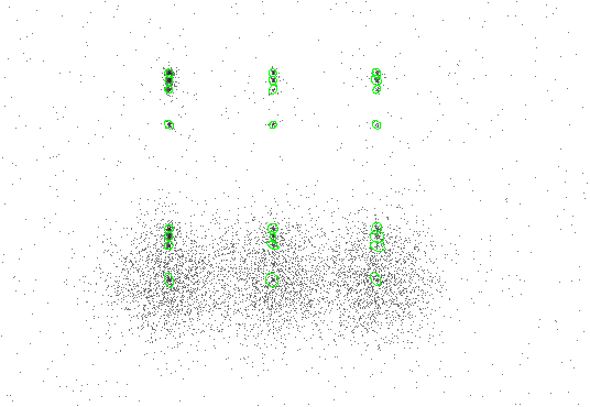
Figure 11.1 shows the data with 3-sigma ellipses from the region file overlaid. Chapter 1, Section 1.4 has instructions on how to display the region file in ds9.
 |
The CIAO tool dmlist is used to for examine the contents of the output file. To see what blocks are in the file:
unix% dmlist example1_out.fits opt=blocks
--------------------------------------------------------------------------------
Dataset: example1_out.fits
--------------------------------------------------------------------------------

     Block Name                          Type         Dimensions
--------------------------------------------------------------------------------
Block    1: PRIMARY                        Null
Block    2: SRCLIST                        Table        26 cols x 24       rows
In the SRCLIST block, there are 26 columns of information for each of the 24 detected sources (one row for each detected source). To list the names of these columns, along with brief column information:
unix% dmlist "example1_out.fits[SRCLIST]" opt=cols

--------------------------------------------------------------------------------
Columns for Table Block SRCLIST
--------------------------------------------------------------------------------

ColNo  Name                 Unit        Type             Range
   1   RA                   deg          Real8          0:      360.0
	Source Right Ascension
   2   DEC                  deg          Real8          -90.0:       90.0
	Source Declination
   3   RA_ERR               deg          Real8          -Inf:+Inf
	Source Right Ascension Error
   4   DEC_ERR              deg          Real8          -Inf:+Inf
	Source Declination Error
   5   POS(X,Y)             pixel        Real8          -Inf:+Inf
	Physical coordinates
   6   X_ERR                pixel        Real8          -Inf:+Inf
	Source X position error
   7   Y_ERR                pixel        Real8          -Inf:+Inf
	Source Y position error
   8   NPIXSOU              pixel        Int4           -
	pixels in source region
   9   NET_COUNTS           count        Real4          -Inf:+Inf
	Net source counts
  10   NET_COUNTS_ERR       count        Real4          -Inf:+Inf
	Error in net source counts
  11   BKG_COUNTS           count        Real4          -Inf:+Inf
	Background counts (scaled to source cell)
  12   BKG_COUNTS_ERR       count        Real4          -Inf:+Inf
	Error in BKG_COUNTS
  13   NET_RATE                          Real4          -Inf:+Inf
	Source count rate (count/exposure map units)
  14   NET_RATE_ERR                      Real4          -Inf:+Inf
	Source count rate error (count/exposure map uni
  15   BKG_RATE                          Real4          -Inf:+Inf
	Background count rate (count/exposure map unit)
  16   BKG_RATE_ERR                      Real4          -Inf:+Inf
	Background count rate error
  17   EXPTIME                           Real4          -Inf:+Inf
	Effective exposure map value (exposure map unit
  18   EXPTIME_ERR                       Real4          -Inf:+Inf
	Effective exposure map error
  19   SRC_SIGNIFICANCE                  Real4          -Inf:+Inf
	Source Significance
  20   PSF_SIZE             pixel        Real4          -Inf:+Inf
	Estimated size of PSF
  21   MULTI_CORREL_MAX                  Int4           -
	1 if source contails 2+ correl maxima
  22   SHAPE                             String[10]
	Shape of source region
  23   R[2]                              Real4(2)       -Inf:+Inf
	Radii of source region source
  24   ROTANG               deg          Real4          0:      180.0
	Rotation angle of source region
  25   PSFRATIO                          Real4          -Inf:+Inf
	Ratio sqrt(axmax*axmin)/psf_size
  26   COMPONENT                         Int4           -
	Source Number

--------------------------------------------------------------------------------
4:
--------------------------------------------------------------------------------

ColNo    Name
5:    EQSRC(RA_SRC ) = (+0)[deg] +TAN[(-0.0001361)* (POS(X)-(+256.50))]
           (DEC_SRC)   (+0)           (+0.0001361)  (   (Y) (+256.50))
To further examine the contents of the output file, use dmlist to show the position and net counts of each source detection:
unix% dmlist "example1_out.fits[SRCLIST][cols X,Y, NET_COUNTS]" opt=data

--------------------------------------------------------------------------------
Data for Table Block SRCLIST
--------------------------------------------------------------------------------

ROW    POS(X,Y)                                 NET_COUNTS

     1 (      251.9739130435,      268.6478260870)       173.5043029785
     2 (      251.8786407767,      309.1310679612)       167.4067993164
     3 (      251.9256198347,      320.4710743802)       312.7768249512
     4 (      252.0469135802,      328.9777777778)       351.6253967285
     5 (      251.9171270718,      451.4972375691)       170.5679016113
     6 (      251.7078651685,      492.3539325843)       155.3647460938
     7 (      251.8429951691,      503.3381642512)       365.8185424805
     8 (      252.0277777778,      511.8636363636)       350.7105407715
     9          (      373.06250,      268.750)        32.4447364807
    10 (      374.0681818182,      309.5227272727)        29.1281700134
    11 (      373.9565217391,      320.0289855072)        54.2208480835
    12 (      373.9577464789,      329.1690140845)        57.9016990662
    13 (      374.1111111111,      451.1944444444)        34.3589019775
    14 (      374.1818181818,      492.6363636364)        27.9628028870
    15 (      373.7014925373,      503.4776119403)        59.2189598083
    16 (      373.8285714286,      512.0857142857)        62.5913848877
    17 (      494.6417910448,      270.1791044776)        36.3386344910
    18 (      496.5862068966,      319.7356321839)        63.0490913391
    19 (      496.7272727273,      308.3409090909)        26.6807270050
    20 (      495.8470588235,      329.4470588235)        68.9102401733
    21 (      495.6571428571,      451.3714285714)        33.5286636353
    22 (      495.9583333333,      492.5833333333)        20.7489109039
    23 (      495.3918918919,      503.6351351351)        64.2184524536
    24     (      495.9583333333,      511.750)        40.6809768677
The graphical user interface of the CIAO tool Prism is an alternative to the command-line interface of dmlist:
unix% prism example1_out.fits &
This next example illustrates running wavdetect using as input the same Chandra dataset from the first example (see Section 11.2.1), but with a few parameters changed from their defaults. This will cause additional output files to be produced:
In addition, the ellsigma parameter is increased to make the display of detected regions easier to see when displayed.
The input file is the same image used in the first example, and the output files are named similarly (example2_something.fits). We begin by setting all the parameters mentioned:
unix% punlearn wavdetect
unix% pset wavdetect infile = "data/datasetA_acis_img.fits[123:630,109:614]"
unix% pset wavdetect outfile = example2_out.fits
unix% pset wavdetect scellfile = example2_scell.fits
unix% pset wavdetect imagefile = example2_image.fits
unix% pset wavdetect defnbkgfile = example2_defnbkg.fits
unix% pset wavdetect regfile = example2_out.reg
unix% pset wavdetect ellsigma = 5
unix% pset wavdetect verbose = 4
unix% pset wavdetect log = yes
DM syntax is used to specify only a portion of the file for input (i.e. [123:630,109:614]); see Chapter 1, Section 1.3.3 for further information about DM syntax usage with
A region file named example2_out.reg will be produced, and the size of the output source ellipses is increased to 5-sigma. The verbosity of log information is changed to 4 and will be recorded in wrecon.log and wtransform.log.
unix% wavdetect
Input file name (data/datasetA_acis_img.fits[123:630,109:614]):
Output source list file name (example2_out.fits):
Output source cell image file name (example2_scell.fits):
Output reconstructed image file name (example2_image.fits):
Output normalized background file name (example2_defnbkg.fits):
unix%
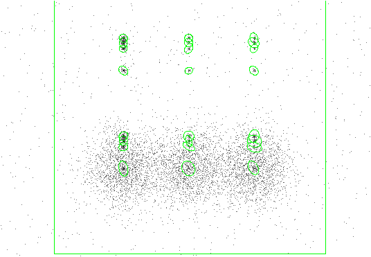
The results are shown in Figure 11.2. Each detection has a 5-sigma ellipse overlay, since ellsigma was set to 5.
 |
unix% dmlist example2_out.fits opt=blocks
--------------------------------------------------------------------------------
Dataset: example2_out.fits
--------------------------------------------------------------------------------

     Block Name                          Type         Dimensions
--------------------------------------------------------------------------------
Block    1: PRIMARY                        Null
Block    2: SRCLIST                        Table        26 cols x 24       rows
The SRCLIST block looks the same as Example 11.2.1: 26 columns of information for each of the 18 detected sources.
unix% more wrecon.log
reading data image
Input image file: data/datasetA_acis_img.fits[123:630,109:614]
Input correlation maxima stack: ./wd_srclist_stk
Input correlation image stack: ./wd_correl_stk
Input background stack: ./wd_nbkg_stk
Input exposure map map:
.
.

unix% more wtransform.log
input file: data/datasetA_acis_img.fits[123:630,109:614]
exposure file:
correlation maxima output stack: ./wd_srclist_stk
correlation image output stack: ./wd_correl_stk
normalized background output stack: ./wd_nbkg_stk
plain background output stack: none
threshold output stack: none
Map is multiplied by time factor 0.000000
.
.
This first example illustrates running wavdetect using a Chandra ACIS dataset of 3C 295 as input; see Chapter 2, Section 2.2 for further information about this dataset.
All parameters are kept at defaults, except for:
Set the parameters:
unix% punlearn wavdetect
unix% pset wavdetect infile = \
"data/acisf00578N002_evt2.fits[(x,y)=rotbox(4114,4232,512,512,0)][ccd_id=7]"
unix% pset wavdetect outfile = example1_out.fits
unix% pset wavdetect scellfile = example1_scell.fits
unix% pset wavdetect imagefile = example1_image.fits
unix% pset wavdetect defnbkgfile = example1_defnbkg.fits
unix% pset wavdetect regfile = example1_out.reg
unix% pset wavdetect ellsigma = 5
DM syntax is used to specify only a portion of the file for input (i.e. [(x,y)=rotbox(4114,4232,512,512,0)]); see Chapter 1, Section 1.3.3 for further information about DM syntax usage with wavdetect .
unix% wavdetect
Input file name (data/acisf00578N002_evt2.fits[(x,y)=rotbox(4114,4232,512,512,0)][ccd_id=7]):
Output source list file name (example1_out.fits):
Output source cell image file name (example1_scell.fits):
Output reconstructed image file name (example1_image.fits):
Output normalized background file name (example1_defnbkg.fits):
unix%
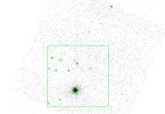
The results are shown in Figure 11.3.
 |
This next example illustrates running wavdetect using as input the same Chandra dataset, but utilizing an exposure map. In this example, wavdetect will be run twice for comparison: with and without an exposure map.
Since we want to utilize an image exposure map, the data must be binned into an image. The dmcopy tool is used to create an image of chip S3 blocked by a factor of 2:
unix% punlearn dmcopy
unix% dmcopy \
"data/acisf00578N002_evt2.fits[ccd_id=7][bin x=::2,y=::2][(x,y)=rotbox(4114,4232,512,512,0)]" \
acisf00578N002_evt2_ccdid7_imgbin2_reg1.fits
An exposure map to match this image was generated following the CIAO thread, "Compute Single Chip ACIS Exposure Map":
http://cxc.harvard.edu/ciao/threads/expmap_acis_single/
unix% punlearn asphist
unix% asphist \
      infile="pcadf052378346N002_asol1.fits[@data/acisf00578N002_evt2.fits[GTI7]]" \
      outfile="asphist_7.fits" evtfile="data/acisf00578N002_evt2.fits" mode="h"

unix% punlearn mkinstmap
unix% mkinstmap outfile="instmap_0.6kev_7.fits" monoenergy="0.6" \
      pixelgrid="1:1024:#1024,1:1024:#1024" obsfile="asphist_7.fits[asphist]" \
      detsubsys="ACIS-7" mode="h"

unix% punlearn mkexpmap
unix% mkexpmap asphistfile="asphist_7.fits" outfile="expmap_0.6kev_7_reg1.fits" \
      instmapfile="instmap_0.6kev_7.fits" normalize="no" \
      xygrid="3857.5:4371.5:#257,3975.5:4489.5:#257" mode="h"
The resulting file is named expmap_0.6kev_7_reg1.fits.
First, wavdetect is run without an exposure map:
Set the necessary parameters:
unix% punlearn wavdetect
unix% pset wavdetect infile = "acisf00578N002_evt2_ccdid7_imgbin2_reg1.fits"
unix% pset wavdetect outfile = example2a_out.fits
unix% pset wavdetect scellfile = example2a_scell.fits
unix% pset wavdetect imagefile = example2a_image.fits
unix% pset wavdetect defnbkgfile = example2a_defnbkg.fits
unix% pset wavdetect regfile = example2a_out.reg
unix% pset wavdetect ellsigma = 5
All other parameters are left at their default values.
unix% wavdetect
Input file name (acisf00578N002_evt2_ccdid7_imgbin2_reg1.fits):
Output source list file name (example2a_out.fits):
Output source cell image file name (example2a_scell.fits):
Output reconstructed image file name (example2a_image.fits):
Output normalized background file name (example2a_defnbkg.fits):
unix%
Next, wavdetect is run with an exposure map:
unix% punlearn wavdetect
unix% pset wavdetect infile = "acisf00578N002_evt2_ccdid7_imgbin2_reg1.fits"
unix% pset wavdetect outfile = example2b_out.fits
unix% pset wavdetect scellfile = example2b_scell.fits
unix% pset wavdetect imagefile = example2b_image.fits
unix% pset wavdetect defnbkgfile = example2b_defnbkg.fits
unix% pset wavdetect expfile = expmap_0.6kev_7_reg1.fits
unix% pset wavdetect regfile = example2b_out.reg
unix% pset wavdetect ellsigma = 5
unix% pset wavdetect expfile = expmap_0.6kev_7_reg1.fits
One additional parameter is used for the exposure map case:
unix% wavdetect
Input file name (acisf00578N002_evt2_ccdid7_imgbin2_reg1.fits):
Output source list file name (example2b_out.fits):
Output source cell image file name (example2b_scell.fits):
Output reconstructed image file name (example2b_image.fits):
Output normalized background file name (example2b_defnbkg.fits):
unix%
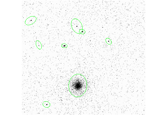
The results of both runs are shown in Figure 11.4. The use of an exposure map with wavdetect improves source property estimates; the detections are the same regardless of whether an exposure map was used. The detections are only affected in the case where the sources exist in an area for which the exposure map has a relative value less than expthresh .
 |
The calculated source properties, however, are improved when an exposure map is supplied to wavdetect . For example, the NET_RATE column in the output will be different because the output values must be divided by the exposure time to obtain true rates with wavdetect .
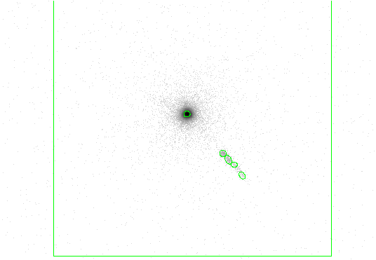
This example illustrates running wavdetect using a Chandra HRC-I dataset of 3C 273 as input; see Chapter 2, Section 2.3 for further information about this dataset.
Set the usual parameters:
unix% punlearn wavdetect
unix% pset wavdetect infile = \
"data/hrcf00461N003_evt2.fits[EVENTS][(x,y)=rotbox(16488.2,16285.8,512,512,0)]"
unix% pset wavdetect outfile = example1_out.fits
unix% pset wavdetect scellfile = example1_scell.fits
unix% pset wavdetect imagefile = example1_image.fits
unix% pset wavdetect defnbkgfile = example1_defnbkg.fits
unix% pset wavdetect regfile = example1_out.reg
unix% pset wavdetect ellsigma = 2
DM syntax is used to specify only a portion of the file for input (i.e. [(x,y)=rotbox(16488.2,16285.8,512,512,0)]); see Chapter 1, Section 1.3.3 for further information about DM syntax usage with wavdetect .
unix% wavdetect
Input file name (data/hrcf00461N003_evt2.fits[EVENTS][(x,y)=rotbox(16488.2,16285.8,512,512,0)]):
Output source list file name (example1_out.fits):
Output source cell image file name (example1_scell.fits):
Output reconstructed image file name (example1_image.fits):
Output normalized background file name (example1_defnbkg.fits):
unix%
Note that the parameter settings made previously using pset are shown when the prompt for the required parameters appears, and that these settings should be accepted by hitting the <RETURN> key.
The results are shown in Figure 11.5.
 |
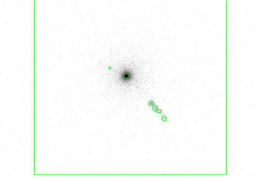
he previous example is repeated, using additional wavdetect scales. Increasing the number of scales means that additional transforms will be computed.
unix% punlearn wavdetect
unix% pset wavdetect infile = \
"data/hrcf00461N003_evt2.fits[EVENTS][(x,y)=rotbox(16488.2,16285.8,512,512,0)]"
unix% pset wavdetect outfile = example2_out.fits
unix% pset wavdetect scellfile = example2_scell.fits
unix% pset wavdetect imagefile = example2_image.fits
unix% pset wavdetect defnbkgfile = example2_defnbkg.fits
unix% pset wavdetect regfile = example2_out.reg
unix% pset wavdetect ellsigma = 2
unix% pset wavdetect scales = "1.0 2.0 4.0 8.0 16.0"
The scales parameter is changed to use five different wavelet radii.
unix% wavdetect
Input file name (data/hrcf00461N003_evt2.fits[EVENTS][(x,y)=rotbox(16488.2,16285.8,512,512,0)]):
Output source list file name (example2_out.fits):
Output source cell image file name (example2_scell.fits):
Output reconstructed image file name (example2_image.fits):
Output normalized background file name (example2_defnbkg.fits):
unix%
The results are shown in Figure 11.6.
 |
cxchelp@head.cfa.harvard.edu