Next: 5. False Detection Rates Up: The Detect Reference Manual Previous: 3. Comparison of Detect Contents
This section highlights some frequently used celldetect parameters. Similar parameters and their description have been grouped together. Chapter 7 has information on each celldetect parameter in alphabetical order.
The input FITS file can an event list or an image. CIAO Data Manipulation (DM) syntax may be used in the input file specification, as explained in Chapter 1, Section 1.3.3.
The current maximum size allowed for an image is 2048![]() 2048, but
an event list may occupy a larger spatial region. For event list
datasets larger than 2048
2048, but
an event list may occupy a larger spatial region. For event list
datasets larger than 2048![]() 2048 (as given by TLMIN, TLMAX),
celldetect may use the "recursive blocking scheme": First the inner
2048
2048 (as given by TLMIN, TLMAX),
celldetect may use the "recursive blocking scheme": First the inner
2048![]() 2048 pixel region of the dataset is searched for sources,
then the inner 4096
2048 pixel region of the dataset is searched for sources,
then the inner 4096![]() 4096 pixel region (excluding the area
already analyzed) is blocked by 2 and searched for sources, then the
inner 8192
4096 pixel region (excluding the area
already analyzed) is blocked by 2 and searched for sources, then the
inner 8192![]() 8192 is blocked by 4, etc. , until TLMIN, TLMAX
is reached. For each consecutive search, the portion of the data that
has already been searched for sources in higher resolution is skipped,
i.e. only one blocking factor is used for each region of the dataset.
4.1For the recursive blocking scheme to operate, fixedcell must be
set to zero and point spread function (PSF) information must be
supplied via psftable (since celldetect will not examine a
dataset past the radius for which PSF information is available).
By default, both fixedcell and psftable are properly set
for recursive blocking of Chandra data.
8192 is blocked by 4, etc. , until TLMIN, TLMAX
is reached. For each consecutive search, the portion of the data that
has already been searched for sources in higher resolution is skipped,
i.e. only one blocking factor is used for each region of the dataset.
4.1For the recursive blocking scheme to operate, fixedcell must be
set to zero and point spread function (PSF) information must be
supplied via psftable (since celldetect will not examine a
dataset past the radius for which PSF information is available).
By default, both fixedcell and psftable are properly set
for recursive blocking of Chandra data.
The outfile parameter is used to provide a name for the output file. The kernel parameter controls the output format; the default is for the output file to have the same format as the input file. If autonaming is used (i.e. "outfile=."), then the output file will be named "<infile_root>_src".
The detection threshold, thresh , is the signal-to-noise (S/N) cutoff for source detection, and should be set to a value of 3 (the default) or 4, particularly for the initial run.
If the findpeaks parameter is set to no, then the source list will consist of all detection cells which exceeded the S/N threshold (often resulting in single source being identified multiple times). If findpeaks is set to yes (the default), then adjacent detections are recognized as a single source and the cell with the largest S/N appears in the source list.
If centroid is set to yes (the default), then the source list will be based on the source centroid. In addition, the major and minor axes of the events distribution are calculated as well as the position angle of the major axis. However, if centroid is set to no, then the center pixel of a source's detect cell is reported as the location of the source.
In addition to the output source list (outfile ), the user may choose to have an ASCII source region file written by specifying a filename in regfile parameter. If autonaming is used (i.e. "regfile=."), then the source regions output file will be named "<infile_root>_reg".
This region file is useful for subsequent input into ds9, particularly to overlay region markers over each detection; see Chapter 1, Section 1.4 for details.
The size of the elliptical source regions in both of the source region files is controlled via the ellsigma parameter. This parameter is a multiplicative factor applied to sigma, the standard deviation of the distribution, to scale the major and minor axes of the ellipses for each source detection. This feature is included so that the graphics overlay may be made more visible; it is does not affect the detections themselves, only the display of the regions.
By default the value for ellsigma is 3, but a larger value is often helpful.
In celldetect , there are three options for computing the background count for a detect cell:
For local detect (option 5), the size of
the background frame is calculated by multiplying the detect cell size
by ![]() , and then rounding it up or down to the closest number
of the same parity as the detect cell size. This acheives two goals:
the area of the background frame is roughly the same as the area of
the detect cell, and the background frame is centered on the same
location as the detect frame.
, and then rounding it up or down to the closest number
of the same parity as the detect cell size. This acheives two goals:
the area of the background frame is roughly the same as the area of
the detect cell, and the background frame is centered on the same
location as the detect frame.
For options 5b and 5c, the background frame is the same as the detect cell. If a background map is provided, then the background value will be obtained from that map, using the same pixels as the detect cell.
celldetect compensates for the larger Chandra PSF off-axis by using a "variable cell size" technique, which increases the size of the detect cell with off-axis distance. The PSF information used by celldetect is contained in a Chandra calibration file distributed with CIAO ; the location is given by the value of the psftable parameter, which points by default to the appropriate Chandra calibration PSF file.
The Chandra HRC and ACIS detectors are the sole combinations in the PSF library file used by celldetect ; information for other missions is not provided. celldetect can only utilize the variable cell size procedure if the following keywords are present in the input Chandra data file (infile ): TELESCOP, INSTRUMENT, DETNAM, GRATING, RA_NOM, and DEC_NOM. If any of the keywords are missing, the tool cannot calculate the appropriate cell size and fixedcell needs to be specified instead.
The selection of a particular PSF size is governed by the energy band eband parameter [keV], since the Chandra PSF is a function of energy. By default the energy band is set to 1.4967 keV.
celldetect also uses an encircled energy percentage value, given by the eenergy parameter, in concert with the calibration PSF file. This value is the percentage of PSF energy to be encircled by the detect cell, expressed as a fraction of 1.0 (default is 0.8). The eenergy is a key parameter for detecting off-axis sources, and users are urged to experiment with other values.
By default, celldetect calculates the off-axis angle using the nominal pointing of the data file as the origin. Users may change this behavior by setting offsets to any numerical values (using the xoffset and yoffset parameters); these offsets provide the location of the optical axis with respect to the center of the data file. A typical scenario in which the user may select to use offsets is when the data file is a sum of two or more observations with different pointings. The nominal pointing in such a data file is usually poorly defined and the off-axis angle could be calculated from an undesired origin, leading to suboptimal selection of the detect cell size.
If a filename is provided for the cellfile parameter, then one or more images are created which contain the detect cell size at each pixel location (see Example 4.2.2). If autonaming is used (i.e. "cellfile=."), then the output stack file will be named "<infile_root>_cell".
celldetect has a fixed cell size option, where the detect cell size is kept constant for the entire dataset. Choose the cell size in pixels by setting the fixedcell parameter; allowed values are 1 or an integer divisible by 3. Setting fixedcell to a non-zero value effectively disables the parameters related to celldetect 's variable cell size functionality: psftable , eenergy , eband , xoffset , and yoffset parameters.
If celldetect is to be run on non-Chandra data, supply a value for fixedcell .
Fixed cell size is also useful for extended source detection. It is well known that local detect methods are not very useful for significantly extended sources. To overcome this limitation, the user may either set fixedcell to a size sufficient to match the expected size of an extended source, or employ a background map (or fixed value for the background) instead of using local detect.
To minimize spurious detections along detector edges, one or more exposure maps may be supplied. The expstk parameter takes a stack of exposure map filenames; sse "ahelp stack'' for more information. Each of the exposure map files should have appropriate binning to match celldetect 's recursive blocking (i.e. binning by 2, 4, 8, ...). Exposure maps only work with the local detect procedure. In addition, they do not work with the convolution option.
The expratio parameter is the ratio of the average exposure of the background frame to the average exposure in the detect cell. Exposure maps supplied by the user are used in conjunction with the expratio parameter. For expratio values other than 0, exposure maps must be supplied in the expstk parameter. Detections for sources whose ratio falls below the specified expratio value will be suppressed from the source region file (regfile ). However, all detections will be present in the output source list (outfile ), and the column EXPO_RATIO will be created. Recommended expratio values ares between 0.9 and 0.99.
Setting convolve to yes will cause detection to be done using the convolution library instead of sliding cells (the default). This method is much slower, does not work with recursive blocking, and should really only be used when an output S/N map is needed.
The convolve option produces a pixel-by-pixel map of the S/N, which is written to the file specified by snrfile . A S/N value is computed for every pixel in the input dataset, not just for source locations. The file snrfile is then an image of these values. If autonaming is used (i.e. "snrfile=."), then the S/N output file will be named "<infile_root>_snr".
celldetect does not not overwrite existing outputs unless clobber is set to yes.
The verbosity of log information ranges from 0 (none) to 5 (maximum output) and is sent to STDERR (usually the screen). However, if log is set to yes, then the log information will be written to the file celldetect.log.
This first example illustrates running celldetect using a simulated ACIS dataset as input; see Chapter 2, Section 2.1 for further information about this dataset.
As required, the user specifies the following:
None of the parameters are changed from their default values, so:
The background will be estimated from a background frame that surrounds the detect cell, i.e. using the "local detect" procedure.
celldetect will use the "variable cell size" technique, increasing the size of the detect cell with off-axis distance, according to the Chandra calibration PSF information distributed with CIAO . The default encircled energy percentage value and energy band are used. The off-axis angle will be calculated using the nominal pointing of the data file as the origin. An output image file of the cell sizes is not produced.
The S/N cutoff for source detection will be 3. Adjacent detections will be recognized as a single source, and the source list will be based on the source centroid.
No ASCII region file will be produced. The FITS source list will contain a 3-sigma ellipse for each detection.
The pset tool is used to supply the required parameter values (infile and outfile ):
unix% punlearn celldetect
unix% pset celldetect infile = data/datasetA_acis_img.fits
unix% pset celldetect outfile = example1_out.fits
Notice that a path may be include with the filenames. Chapter 1, Section 1.3.1 has further information on manipulating parameters.
If desired, the user may then list the current celldetect parameter settings with plist:
unix% plist celldetect
Parameters for /home/username/cxcds_param/celldetect.par

#
#   celldetect parameter file
#
#
#   input
#
        infile = data/datasetA_acis_img.fits Input file
#
#   output
#
       outfile = example1_out.fits Output source list
       (expstk = )                list of exposure map files
      (regfile = none)            ASCII regions file
#
#   output options
#
       (kernel = default)         Output file format
      (clobber = no)              Overwrite exiting outputs?
#
#   output content/format options
#
       (thresh = 3)               Source threshold
    (findpeaks = yes)             Find local peaks?
     (centroid = yes)             Compute source centroids?
     (ellsigma = 3)               Size of output source ellipses (in sigmas)
     (expratio = 0)               cutoff ratio for source cell exposure variation
#
#   detect cell size parameters
#
    (fixedcell = 0)               Fixed cell size to use (0 for variable cell)
      (xoffset = INDEF)           Offset of x axis from data center
      (yoffset = INDEF)           Offset of y axis from data center
        (eband = 1.4967)          Energy band
      (eenergy = 0.8)             Encircled energy of PSF
     (psftable = ${ASCDS_CALIB}/psfsize20010416.fits -> /soft/ciao/data/psfsize20010416.fits) Table of PSF size data
     (cellfile = )                Output cell size image stack name
#
#   background parameters
#
      (bkgfile = )                Background file name
     (bkgvalue = 0)               Background count/pixel
  (bkgerrvalue = 0)               Background error
#
#   using defaults is recommended here
#
     (convolve = no)              Use convolution?
      (snrfile = )                SNR output file name (for convolution only)
#
#   run log verbosity and content
#
      (verbose = 0)               Log verbosity level
          (log = no)              Make a celldetect.log file?
#
#   mode
#
         (mode = ql)
To execute celldetect , type the name of the tool on the command line:
unix% celldetect
Input file (data/datasetA_acis_img.fits):
Output source list (example1_out.fits):
unix%
The parameter settings are shown in the prompt for each required parameter; these settings may be accepted by hitting the <RETURN> key or changed if desired.
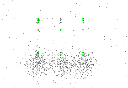
Figure 4.1 shows the data with 3-sigma ellipses from the region file overlaid. Chapter 1, Section 1.4 has instructions on how to display the region file in ds9.
 |
The CIAO tool dmlist is used to for examine the contents of the output file. To see what blocks are in the file:
unix% dmlist example1_out.fits opt=blocks
--------------------------------------------------------------------------------
Dataset: example1_out.fits
--------------------------------------------------------------------------------

     Block Name                          Type         Dimensions
--------------------------------------------------------------------------------
Block    1: PRIMARY                        Null
Block    2: SRCLIST                        Table        31 cols x 18       rows
In the SRCLIST block, there are 31 columns of information for each of the 18 detected sources (one row for each detected source). To list the names of these columns, along with brief column information:
unix% dmlist "example1_out.fits[SRCLIST]" opt=cols

--------------------------------------------------------------------------------
Columns for Table Block SRCLIST
--------------------------------------------------------------------------------

ColNo  Name                 Unit        Type             Range
   1   RA                   deg          Real8          0:      360.0
	Source Right Ascension
   2   DEC                  deg          Real8          -90.0:       90.0
	Source Declination
   3   RA_ERR               deg          Real8          -Inf:+Inf
	Source Right Ascension Error
   4   DEC_ERR              deg          Real8          -Inf:+Inf
	Source Declination Error
   5   POS(X,Y)             pixel        Real8          -Inf:+Inf
	Physical coordinates
   6   X_ERR                pixel        Real8          -Inf:+Inf
	Source X position error
   7   Y_ERR                pixel        Real8          -Inf:+Inf
	Source Y position error
   8   CELLPOS(CELL_X,CELL_Y) pixel        Real8          -Inf:+Inf
	Physical coordinates
   9   DETSIZE              pixel        Int4           -
	source cell size
  10   BKGSIZE              pixel        Int4           -
	background cell size
  11   NPIXSOU              pixel        Int4           -
	pixels in source cell
  12   NPIXBKG              pixel        Int4           -
	pixels in background cell
  13   NET_COUNTS           count        Real4          -Inf:+Inf
	Net source counts
  14   NET_COUNTS_ERR       count        Real4          -Inf:+Inf
	Error in net source counts
  15   BKG_COUNTS           count        Real4          -Inf:+Inf
	Background counts (scaled to source cell)
  16   BKG_COUNTS_ERR       count        Real4          -Inf:+Inf
	Error in BKG_COUNTS
  17   NET_RATE             count/s      Real4          -Inf:+Inf
	Source count rate
  18   NET_RATE_ERR         count/s      Real4          -Inf:+Inf
	Source count rate error
  19   BKG_RATE             count/s      Real4          -Inf:+Inf
	Background count rate
  20   BKG_RATE_ERR         count/s/pixel Real4          -Inf:+Inf
	Background count rate error
  21   EXPTIME              s            Real4          -Inf:+Inf
	Effective exposure time
  22   SNR                               Real4          -Inf:+Inf
	Signal-to-Noise ratio
  23   SHAPE                             String[10]
	Shape of source region
  24   R[2]                              Real4(2)       -Inf:+Inf
	Radii of source region source
  25   ROTANG               deg          Real4          0:      180.0
	Rotation angle of source region
  26   PSFRATIO                          Real4          -Inf:+Inf
	ratio of source ellipse size to PSF size
  27   BLOCK                             Int4           -
	blocking factor
  28   COMPONENT                         Int4           -
	Source Number
  29   EXPO_RATIO                        Real4          -Inf:+Inf
	ratio of average background and detect cell exp
  30   DOUBLE                            Logical
	double detection flag
  31   DOUBLE_ID                         Int4           -
	double source component

--------------------------------------------------------------------------------
4:
--------------------------------------------------------------------------------

ColNo    Name
5:    EQSRC(RA_SRC ) = (+0)[deg] +TAN[(-0.0001361)* (POS(X)-(+256.50))]
           (DEC_SRC)   (+0)           (+0.0001361)  (   (Y) (+256.50))
8:    EQSRC_CELL(RA_CELL_X ) = (+0)[deg] +TAN[(-0.0001361)* (CELLPOS(CELL_X)-(+256.50))]
                (DEC_CELL_Y)   (+0)           (+0.0001361)  (       (CELL_Y) (+256.50))
To further examine the contents of the output file, use dmlist to show the position and net counts of each source detection:
unix% dmlist "example1_out.fits[SRCLIST][cols X,Y, NET_COUNTS]" opt=data

--------------------------------------------------------------------------------
Data for Table Block SRCLIST
--------------------------------------------------------------------------------

ROW    POS(X,Y)                                 NET_COUNTS

     1 (      251.9541284404,      268.8899082569)        80.31250
     2 (      252.0310077519,      309.0387596899)       113.250
     3 (      251.9555555556,      320.9833333333)       123.750
     4 (      252.0196078431,      329.0196078431)       217.8750
     5 (      252.0491803279,      451.7786885246)       106.81250
     6 (      373.8648648649,      320.0540540541)         28.0
     7 (      251.8198757764,      492.4347826087)       148.1428527832
     8 (      251.8598901099,      503.4862637363)       331.8571472168
     9 (      251.9226190476,      511.8779761905)       285.8571472168
    10 (      374.0357142857,      492.1071428571)        25.4285717010
    11 (      373.6935483871,      512.0806451613)        55.5714302063
    12 (      374.2647058824,      451.3235294118)         34.0
    13 (      374.2641509434,      503.4905660377)         44.0
    14       (      495.3666666667,      309.0)        24.8571434021
    15 (      495.6304347826,      318.7173913043)        33.1428565979
    16 (      495.4923076923,      329.1846153846)        53.4285697937
    17 (      495.6935483871,      503.7419354839)        54.2857131958
    18          (      495.9750,      511.3750)        32.2857131958
The graphical user interface of the CIAO tool Prism is an alternative to the command-line interface of dmlist:
unix% prism example1_out.fits &
This next example illustrates running celldetect using as input the same Chandra dataset from the first example (see Section 4.2.1), but with a few parameters changed from their defaults. This will cause additional output files to be produced:
In addition, the ellsigma parameter is increased to make the display of detected regions easier to see when displayed.
The input file is the same image used in the first example, and the output file is to be named example2_out.fits. We begin by setting all the parameters mentioned:
unix% punlearn celldetect
unix% pset celldetect infile = "data/datasetA_acis_img.fits"
unix% pset celldetect outfile = example2_out.fits
unix% pset celldetect regfile = example2_out.reg
unix% pset celldetect ellsigma = 5
unix% pset celldetect cellfile = example2_cellfile.stack
unix% pset celldetect verbose = 4
unix% pset celldetect log = yes
A region file named example2_out.reg will be produced, and the size of the output source ellipses is increased to 5-sigma. The output cell size image stack file, which contains information about the detect cell sizes used, will be named example2_cellfile.stack. Finally, the verbosity of log information is changed to 4 and will be recorded in celldetect.log.
unix% celldetect
Input file (data/datasetA_acis_img.fits):
Output source list (example2_out.fits):
unix%
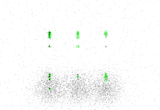
The results are shown in Figure 4.2. Each detection has a 5-sigma ellipse overlay, since ellsigma was set to 5.
 |
unix% dmlist example2_out.fits opt=blocks

--------------------------------------------------------------------------------
Dataset: example2_out.fits
--------------------------------------------------------------------------------

     Block Name                          Type         Dimensions
--------------------------------------------------------------------------------
Block    1: PRIMARY                        Null
Block    2: SRCLIST                        Table        31 cols x 18       rows
The SRCLIST block looks the same as Example 4.2.1: 31 columns of information for each of the 18 detected sources.
unix% more example2_cellfile.stack
datasetA_acis_img_cell_1.fits
There is only one filename in this case, but multiple files may be created, depending on how celldetect is run. This image may be viewed using ds9:
unix% ds9 datasetA_acis_img_cell_1.fits &
unix% more celldetect.log
input file: data/datasetA_acis_img.fits[123:630,109:614]
output file: example2_out.fits
ASCII source regions file: example2_out.reg
creating cell size table
reading data image
creating candidate source list
cell size 3
cell size 6
cell size 9
cell size 12
Writing out cell file: datasetA_acis_img_cell_1.fits
This next example illustrates running celldetect using as input the same Chandra dataset from the first two examples (see Section 4.2.1 and Section 4.2.2). The following parameters will be used:
We begin by setting all the parameters just mentioned:
unix% punlearn celldetect
unix% pset celldetect infile = "data/datasetA_acis_img.fits"
unix% pset celldetect outfile = example3_out.fits
unix% pset celldetect regfile = example3_out.reg
unix% pset celldetect ellsigma = 5
unix% pset celldetect thresh = 2.5
All other parameters are left at their default values.
unix% celldetect
Input file (data/datasetA_acis_img.fits):
Output source list (example3_out.fits):
unix%
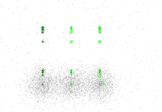
Figure 4.3 shows the data overlaid with 5-sigma ellipses.
 |
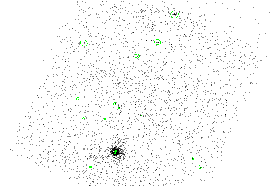
This first example illustrates running celldetect using a Chandra ACIS dataset of 3C 295 as input; see Chapter 2, Section 2.2 for further information about this dataset.
All parameters are kept at defaults, except for:
Set the parameters:
unix% punlearn celldetect
unix% pset celldetect infile = \
"data/acisf00578N002_evt2.fits[EVENTS][ccd_id=7]"
unix% pset celldetect outfile = example1_out.fits
unix% pset celldetect regfile = example1_out.reg
unix% pset celldetect ellsigma = 5
DM syntax is used to select the chip of interest for input (i.e. [ccd_id=7]); see Chapter 1, Section 1.3.3 for further information about DM syntax usage with celldetect .
unix% celldetect
Input file (data/acisf00578N002_evt2.fits[EVENTS][ccd_id=7]):
Output source list (example1_out.fits):
unix%
The results are shown in Figure 4.4.
 |
This next example illustrates running celldetect on chip S1 (ccd_id=5) of dataset B. In this example, celldetect will be run twice for comparison: with and without an exposure map.
Since we want to utilize an image exposure map, the data must be binned into an image. The dmcopy tool is used to create an image of chip S1 blocked by a factor of 4:
unix% punlearn dmcopy
unix% dmcopy "data/acisf00578N002_evt2.fits[ccd_id=5][bin x=::4,y=::4]" \
"acisf00578N002_evt2_ccdid5_imgbin4.fits"
An exposure map to match this image was generated following the CIAO thread, "Compute Single Chip ACIS Exposure Map":
http://cxc.harvard.edu/ciao/threads/expmap_acis_single/
unix% punlearn asphist
unix% asphist \
      infile="pcadf052378346N002_asol1.fits[@data/acisf00578N002_evt2.fits[GTI5]]" \
      outfile="asphist_5.fits" evtfile="data/acisf00578N002_evt2.fits" mode="h"

unix% punlearn mkinstmap
unix% mkinstmap outfile="instmap_1.8kev_5.fits" monoenergy="1.8" \
      pixelgrid="1:1024:#1024,1:1024:#1024" obsfile="asphist_5.fits[asphist]" \
      detsubsys="ACIS-5" mode="h"

unix% punlearn mkexpmap
unix% mkexpmap asphistfile="asphist_5.fits" outfile="expmap_1.8kev_5_2048.fits" \
      instmapfile="instmap_1.8kev_5.fits" normalize="no" \
      xygrid="0.5:8192.5:#2048,0.5:8192.5:#2048" mode="h"
The resulting file is named expmap_1.8kev_5_2048.fits.
First, celldetect is run without an exposure map:
Set the necessary parameters:
unix% punlearn celldetect
unix% pset celldetect infile = "acisf00578N002_evt2_ccdid5_imgbin4.fits"
unix% pset celldetect outfile = example2a_out.fits
unix% pset celldetect regfile = example2a_out.reg
unix% pset celldetect ellsigma = 5
All other parameters are left at their default values.
unix% celldetect
Input file (acisf00578N002_evt2_ccdid5_imgbin4.fits):
Output source list (example2a_out.fits):
unix%
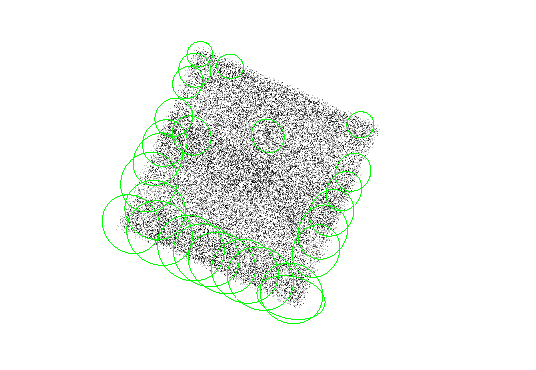
The results are shown in Figure 4.5.
 |
Next, celldetect is run with an exposure map:
unix% punlearn celldetect
unix% pset celldetect infile = "acisf00578N002_evt2_ccdid5_imgbin4.fits"
unix% pset celldetect outfile = example2b_out.fits
unix% pset celldetect regfile = example2b_out.reg
unix% pset celldetect ellsigma = 5
unix% pset celldetect expstk="expmap_1.8kev_5_2048.fits"
unix% pset celldetect expratio=0.9
Two additional parameters are used for the exposure map case:
unix% celldetect
Input file (acisf00578N002_evt2_ccdid5_imgbin4.fits):
Output source list (example2b_out.fits):
unix%
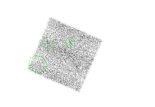
The results are shown in Figure 4.6.
 |
This example illustrates running celldetect using a Chandra HRC-I dataset of 3C 273 as input; see Chapter 2, Section 2.3 for further information about this dataset.
Set the usual parameters:
unix% punlearn celldetect
unix% pset celldetect infile = \
"data/hrcf00461N003_evt2.fits[EVENTS][(x,y)=rotbox(16488.2,16285.8,512,512,0)]"
unix% pset celldetect outfile = example1_out.fits
unix% pset celldetect regfile = example1_out.reg
unix% pset celldetect ellsigma = 5
DM syntax is used to specify only a portion of the file for input (i.e. [(x,y)=rotbox(16488.2,16285.8,512,512,0)]); see Chapter 1, Section 1.3.3 for further information about DM syntax usage with celldetect .
unix% celldetect
Input file (data/hrcf00461N003_evt2.fits[EVENTS][(x,y)=rotbox(16488.2,16285.8,512,512,0)]):
Output source list (example1_out.fits):
unix%
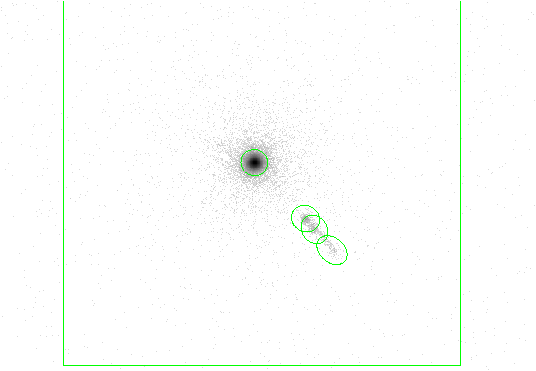
The results are shown in Figure 4.7.
 |
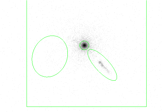
The previous example is repeated, but the fixed cell size option is used, meaning the detect cell size is kept constant for the entire dataset.
unix% punlearn celldetect
unix% pset celldetect infile = \
"data/hrcf00461N003_evt2.fits[EVENTS][(x,y)=rotbox(16488.2,16285.8,512,512,0)]"
unix% pset celldetect outfile = example2_out.fits
unix% pset celldetect regfile = example2_out.reg
unix% pset celldetect ellsigma = 5
unix% pset celldetect fixedcell = 60
The fixedcell parameter to match the expected size of the extended emission sources.
unix% celldetect
Input file (data/hrcf00461N003_evt2.fits[EVENTS][(x,y)=rotbox(16488.2,16285.8,512,512,0)]):
Output source list (example2_out.fits):
unix%
The results are shown in Figure 4.8.
 |
cxchelp@head.cfa.harvard.edu