Gregory-Laredo Variability Algorithm for Chandra Data

Previous   Contents   Next


Gregory-Laredo Variability Algorithm for Chandra Data

Reprinted by permission from ADASS XV Proceedings (Escorial, Spain, 2005) ASP Conf. Ser., G. Gabriel, C. Arviset, D. Ponz, and E. Solano, eds.

Introduction

We describe using the Gregory-Loredo algorithm (Gregory & Loredo 1992) to detect temporal variability in sources identified in the CXC L3 pipeline (Evans et al. 2006), based on the event files. Briefly, N events are binned in histograms of m bins, where m runs from 2 to mmax. The algorithm is based on the likelihood of the observed distribution n1 n2, ..., nm occurring. Out of a total number of mN possible distributions the multiplicity of this particular one is N!/(n1! . n2! . ... . nm!). The ratio of this multiplicity to the total number provides the probability that this distribution came about by chance. Hence the inverse is a measure of the significance of the distribution. In this way we calculate an odds ratio for m bins versus a flat light curve. The odds are summed over all values of m to determine the odds that the source is time-variable.
The method works very well on event data and is capable to deal with data gaps. We have added the capability to take into account temporal variations in effective area. As a byproduct, it delivers a light curve with optimal resolution.

Although the algorithm was developed for detecting periodic signals, it is a perfectly suitable method for detecting plain variability by forcing the period to the length of the observation.

We have implemented the G-L algorithm as a standard C program, operating on simple ASCII files for ease of experimentation. Input data consist of a list of event times and, optionally, good time intervals with, optionally, normalized effective area.
Two output files are created: odds ratios as a function of m and a light curve file.
If mmax is not explicitly specified, the algorithm is run twice. The first time all values of m are used, up to the minimum of 3000 and (te - tb) /50; i.e., variability is considered for all time scales down to 50s, which is about 15 times the most common ACIS frame time. The sum of odds S(m) = O(i) / (i - mmin + 1), where i = mmin ... m, is calculated as a function of m and its maximum is determined. Then the algorithm is run again with mmax set to the highest value of m for which S(m) > max(S) / e. In addition to the total odds ratio O the corresponding probability P of a variable signal is calculated.
The light curve that is generated by the program essentially consists of the binnings weighed by their odds ratios and represents the most optimal resolution for the curve. The standard deviation σ is provided for each point of the curve.
There is an ambiguous range of probabilities: 0.5 < P < 0.9, and in particular the range between 0.5 and 0.67 (above 0.9 all is variable, below 0.5 all is non-variable). For this range we have developed a secondary criterion, based on the light curve, its average σ, and the average count rate. We calculate the fractions f3 and f5 of the light curve that are within 3σ and 5σ, respectively, of the average count rate. If f3 > 0.997 AND f5 = 1.0 for cases in the ambiguous probability range, the source is deemed to be non-variable.

Finally, the program assigns a variability index (see Table 3).

Test Results and Analysis

The program was run on all 118 sources found by the program wavdetect in Chandra ObsId 635. The total time span of the observation was 102 ks and the sources varied between 5 and 24000 counts. The average time to run the program was 1.5 s per source. 71 sources were found to be variable with an odds ratio > 1.0 (probability > 0.5). Visual inspection of the light curves of all 118 sources found 54 that are variable, though there are a few borderline cases on either side of the divide.

Analysis

Table 3 summarizes the number of variable sources detected,
Variability Index
Condition
Comment
0
0 < P < 0.5
Definitely not variable
1
0.5 < P < 0.67
and f
3 > 0.997 and f5 = 1.0
Not considered variable
2
0.67 < P < 0.9
and f
3 > 0.997 and f5 = 1.0
Probably not variable
3
0.5 < P < 0.6
May be variable
4
0.6 < P < 0.67
Likely to be variable
5
0.67 < P < 0.9
Considered variable
6
0.9 < P and O < 2.0
Considered variable
7
2 < O < 4
Considered variable
8
4 < O < 10
Considered variable
9
10 < O < 30
Considered variable
10
30 < O
Considered variable

TABLE 3: Variability index.
the false, and the missed detections, as a function of odds ratio and probability range.
Using G-L just by itself is problematic in the probability range 0.5-0.9, considering the required trade-off between missed detections and false detections. We solved this problem, as described above, by designing the secondary criterion that is based on the fraction of the light curve within 3σ and 5σ. The final result is that three borderline variable sources are missed (with emphasis on borderline), but there are no spurious detections. However, any user who is concerned about missing potential candidates should be encouraged to inspect all sources with a variability index greater than 0.
The G-L algorithm, as expected, is pleasantly insensitive to the shape of the light curve.
The light curves (and the 3σ curves), in providing precisely the desired resolution, are of the kind that we would want to include in the product package.
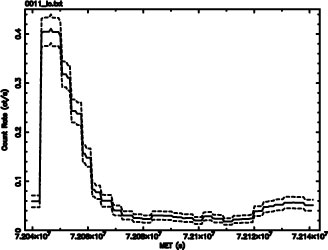
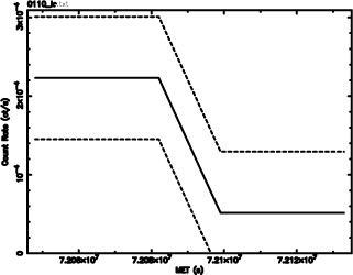
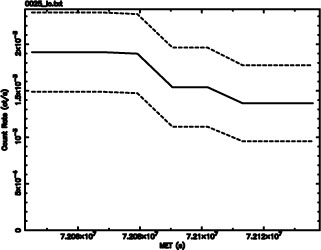
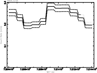
Figs. 24 - 26 provide a typical cross-section of the different types of cases. Dashed lines represent the 3σ curves. Fig. 27 shows one of the cases that cannot very well be handled by simple statistics: it fails all criteria, but there appears to be a definite trend; however, we do not consider the source variable.
The tests have also brought to light the issue of time-variable exposure (or effective area). It appears in a number of sources with characteristic times that are harmonics of one of Chandra’s two dither periods (707 and 1000 s). Our tests show that this can be properly taken care of by providing the program with normalized effective area as a function of time.

FIGURE 24: Source 3 (24093 counts). Even though the SNR is high, the resolution of the light curve is fairly low since higher resolution is not warranted by its shape.


Odds ratio range
Probability range
Good
detections
False
detections
Missed with secondary criterion
False with secondary criterion
1.0 - 2.0
0.5 - 0.67
2
7
1
0
2.0 - 9.0
0.67 - 0.9
5
10
2
0
> 9.0
> 0.9
47
0
0
0

TABLE 4: Detection results.

FIGURE 25: Source 11 (8697 counts). The timescale of the changes in this source are very much shorter than in source 3; hence the resolution is higher.


FIGURE 26: Source 110 (14 counts). A low count rate, but variable, nevertheless.


FIGURE 27: Source 25 (170 counts). This is an example of a borderline case where there is no statistically significant change while there is yet an unmistakable trend. I still would not consider this source variable.
Conclusion

We conclude that G-L provides a robust algorithm for detecting temporal variability that is insensitive to the type and shape of variability and that takes properly into account the uncertainties in the count rate, requiring a statistically significant departure from a flat count rate for it to declare variability. The light curves provided by the program appear to be near-optimal for what we intend to present to users. The addition of the secondary criterion results in a reliable test, though careful users may want to inspect the light curves of all sources with a non-zero variability index.


This work has been supported by NASA under contract NAS 8-03060 to the Smithsonian Astrophysical Observatory for operation of the Chandra X-ray Center. I gratefully acknowledge many useful discussions with Dr. Gregory.

Arnold Rots

References

Evans, I. et al. 2006, ADASS XV
Gregory, P. C. & Laredo, T. J. 1992, ApJ, 398, 146