Our goals are based on well known and critical atomic data issues, and take advantage of physical scaling laws for different atomic processes. The plan is to test ions that represent a range of elements (nuclear charge or Z-scaling), a range of ionization states (isoelectronic sequence scaling), and a range of principal quantum numbers (n scaling).
While we calculate exposure times based on specific lines that we can predict, we note that lines missing in the models, even if individually weak, can contribute significant power as unresolved line complexes. We will place significant constraints on them by summing over wavebands where the weak emission occurs, and comparing the flux to relatively line-free spectral regions. Important weak line complexes include those of the less common elements not in the current codes, and lines from very high n levels.
The three sources have all been studied by a multitude of high energy satellites, and are the brightest sources in their respective temperature ranges. Furthermore, these sources have been studied extensively with EUVE, providing longer wavelength line intensity measurements than will be obtained with AXAF. We have compiled what we consider to be the best available atomic physics models to predict fluxes for emission lines. For the HEG band, we use SPEX; for the LETG band, we combine SPEX; Brickhouse-Raymond-Liedahl; and Raymond-Smith; and Liedahl (1996).
The emission measure distributions are derived from Drake et al. (1995), Brickhouse (1996), and Griffiths (1996) for Procyon, Capella, and HR 1099, respectively. We have used recent calibration AXAF effective area curves to generate emission line count rates.
The useful cut-off for benchmarking is signal-to-noise of 10, which translates into a 3-sigma uncertainty of about 30%. We use signal-to-noise = S/sqrt(S+B), where S is the total number of counts in the line and B is the total number of background counts, including sky, continuum, and unresolved weak line contributions. The sky background is negligible, and for Capella and Procyon there is an insignificant contribution from the continuum. Since the background from weak lines is an issue that has never been addressed, we arbitrarily assume that the background is 20% for the LETG (including high order weak line flux). For Capella in the HEG we ignore the background, while for HR 1099 we calculate the continuum flux separately. The critical spectral region for benchmarking is around 10 Å, where the continuum flux per resolution element of HR 1099 is similar to the individual line fluxes. Hence for HR 1099, B ~ S.
Figures3 to 6 show the emission line counts predicted for the proposed exposure times for each source. We require 150 ks for Procyon in the LETG, 100 ks each for LETG and HEG observations of Capella, and 200 ks for HR 1099 with HEG. We do not require the Drake flat for the Procyon observation since only a few strong high order lines will appear. For the Capella calculation we are using the effective areas without the Drake flat; however, that decision will be more informed once the flat performance is better characterized. If the flat is used, the exposure time will need to be increased by 40% above the value shown. The + symbols are used for all emission lines on all plots (and thus appear redundantly for each source); bullet symbols are overplotted to highlight lines of elements or ions of interest. The dotted line represents S/N=10, our cut-off.
Procyon. The Procyon spectrum will primarily be used to benchmark the LETG spectral region (Fig. 3). Since this wavelength region has never been thoroughly studied, the most critical aspect of the Procyon measurements is to provide a high quality spectrum for discovery of new (and ``missing'') lines, line identification and wavelengths through comparison with spectral predictions, and intensity checks on strong lines. While EUVE measurements have explored the overlapping spectral region above 80 Å the spectral resolution of EUVE is significantly less ( E/ Delta E ~ 200 to 400), and a number of scientific results hinge on a good assessment of line blending, particularly for lines measured in the Procyon temperature range.
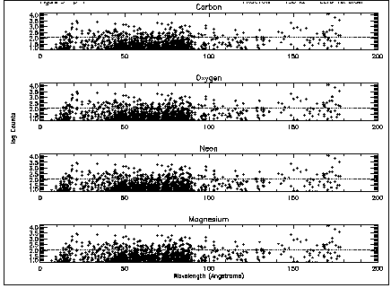
Figure 3. Procyon 1st order lines in the LETG for a 150 ks exposure (no Drake flat). Note the strong lines of Fe IX to XI above 170 Å. The Fe lines between 50 and 100 Å are lines of Fe XV to XVIII. The proposed test of the ionization and recombination balance is to compare the emission measure distribution derived from these lines with those from the other elements. For example, the X-ray lines from O around 20 Å are from O VII and O VIII, while most of the lines above 100 Å are from O V and VI.
The proposed exposure times will provide approximately 160 useful lines with signal-to-noise greater than 10. Even with this seemingly large number of emission lines, the degree of redundancy is modest, with only one or two lines per ion for many of the ions. With even two lines from the same ion, we can begin to test the collisional and radiative excitation rates which are used to calculate relative level populations. Of great interest are the L-shell ions in the intermediate Z range (ions of Ne to Ar) and Fe M-shell emission.
The proposed study of the Procyon spectrum can also provide a unique test of the ionization balance. The dielectronic recombination rates are highly uncertain in general, and with increasing Z the effects of additional inner shell processes are quite controversial. The proposed exposure time is sufficient to compare the ionization balance of O and Fe (from emission measure distributions derived independently with complete coverage) over the temperature range from 106 to 6 x 10⁶ K (we will obtain O V--VIII and Fe IX--XVIII, with Fe XVII in higher order). Of particular concern is the ionization balance around Ne-like Fe XVII. Thus good signal-to-noise in Fe XVIII (the highest ionization state in the Procyon spectrum) provides a critical constraint on the exposure time. In addition, this exposure time allows additional tests of the ionization balance from the intermediate Z ions and tests of strong Ni lines.
Capella. In the LETG band the arguments are similar to those for Procyon, except that Capella emits lines from higher ionization states than Procyon due to its higher temperature (Fig. 4). Thus we will provide a different set of lines, and test ionization balance (Fe XV to XXIII; O VI to VIII) in the range 3 x 10^6 to 1.5 x 10^7 K. The exposure time of 100 ks will need to be increased to 140 ks if this observation is made with the Drake flat.
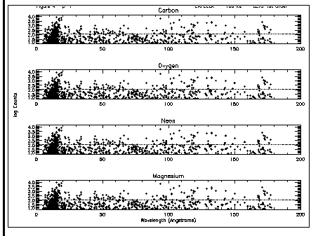
Figure 4. Capella 1st order lines in the LETG for a 100 ks exposure (no Drake flat). The critical ionization balance test is for higher temperatures and thus higher ionization states of Fe.
In the HETG band Capella will provide the critical test of Fe L shell emission from Fe XVII through XIX (Fig. 5). These ions present a difficult challenge for theoretical computation due to their complex electron configurations. The proposed exposure will allow us to test n=4 -> 2 to n=3 -> 2 line ratios of the strongest lines. Emission originating from still higher n levels will be constrained by measurements of total fluxes in narrow bands where numerous weak emission lines are expected.
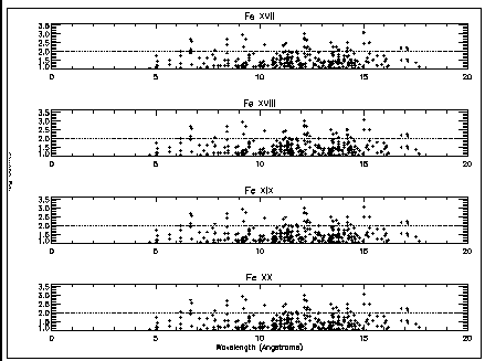
Figure 5. Capella HEG lines for a 100 ks exposure. The critical benchmarking test is the ratio of the n=4 --> 2/n=3 -->2 lines of Fe. As an example, the Fe XVII n=3 --> 2 lines above 13 Å and the n=4 --> 2 lines below 13 Å are obtained. Note that the ``missing'' lines are predicted to be between 11.4 Å and the ionization limit at 9.8 Å. We now believe that the ASCA spectral fit for Capella fails because of the total strength of missing Fe lines in the codes. AXAF will resolve the strong Ne X line shown at 10.24 Å, and additional flux in that band will be summed to compare with models now being computed. Note also that for Fe XX to XXIV the signal-to-noise is not enough.
HR 1099. Since HR 1099 has a harder spectrum than Capella the benchmarking tests of interest are the higher ionization stages of Fe (Fig. 6). Again we take the n=4 -> 2 vs n=3 -> 2 line ratio as the critical test. Since Fe XXIV has been benchmarked with laboratory measurements at the EBIT (Savin et al. 1996) we focus on Fe XXI to Fe XXIII.