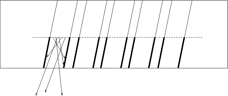
Figure 1: End-Spoiled Zone
HRC uses a two stage Microchannel Plate (MCP) as a part of its detector. Once an X-ray photon entries one of the pores of the first MCP, it creates a cascade of electrons. These electrons fly into multiple pores of the second MCP and the numbers of electrons are farther amplified before reaching to the target where the distribution of electrons is read out.
In this study, we create a three-dimensional simulation model to recreate HRC I readout signal distributions and compared them to actual event data.
The diameter of a pore of HRC I MCP is 10.0μm, and the distance between two centers of adjacent pores is 12.5μm. The length of a MCP pore is about 1,200μm, but in this simulation, the length of an end spoil (ES) zone is a more relevant parameter.
The ES zone is the area of a pore where electrons are not produced by an incoming electron but it is actually absorbed by the wall (see Figure 1). The length of the ES zone is not well known, and in this study, we set the length of ES zone between 0.5 and 3.0 times of the pore diameter (hereafter, ES ratio).
Pores are tilted 6 degree in one direction in the first MCP and in another direction in the second MCP.
After leaving the first stage MCP, electrons are accelerated by the 50V electric field, fly the distance of 127μm, and entire the pores of the second MCP. We assume that the length of the ES zone of the second MCP is the same as that of the first MCP. The distance to the target from the bottom of the second MCP is 4mm, and there is 300V of the electric field between them.
Two MCPs could be overlapped in three possible ways. The first possibility is that pore positions of the both MCPs perfectly match. The second possibility is that the second MCP is shifted in the X direction, and the third possibility is that the second MCP is shifted both in the X and the Y direction (see Figure 2).
The simulations are done in the following ways:
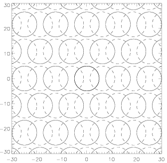
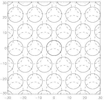
Figures 3a and 4a show two dimensional plots of the electron distributions created by a single X-ray photon for ES ratio = 0.5 and 2.0 case, respectively. Three figures are, left to right, the case that two MCPs are perfectly overlapped, the case that the pores of the second MCP are shifted in the X direction (Figure 2 left), and the case that the pores of the second MCP are shifted both in the X and the Y directions (Figure 2 right).
Figures 3b and 4b are one dimensional electron distributions along the X axis for ES ratio = 0.5 and 2.0, respectively. Three plots are same as the two dimensional case. The unit of the axis is in the pore diameter, and it is centered at the position of the pore of the first MCP. The count is normalized so that the maximum counts is 1.0.
)
)
)
)
)
)
)
)
)
)
)
) .
.
In reality, what we see from HRC is a signal generated by the charge accumulation at the wire mesh at the bottom of the detector. A cascade of electrons created from the second MCP hits equally spaced wires and the charges are collected by these wires. The amount of changes are read out from taps located every 8th wire. In this study, we assume that the distance between two taps is 1.648mm, which is based on a pixel size (6.43μm) and the number of pixels between two taps (256 pixels).
Figure 5 shows the schimatic diaglam of the Cross Grid Charged Detector (CGCD). The diameter of the wire is 100 μm, and spaced 206 μm from the center of one wire to the next. The top grids catches electrons for V axis, and the bottom grids for U axis. The distance between two grids are 400 μm.
The distance between U grids to the reflector is 1.0 mm, and the reflector is biased -50V relative to the U grids. We assume that all reflected back electrons are absoved by the U grids.
To estimate an X-ray location, we need to read the amounts of charges from three adjacent taps with the highest charge accumulation at the center tap. Then the location of the X-ray can be estimated by:
Please see HRC Position Logic (Juda, 1996) for more details.
Figure 6 shows an example simulations with ES ratio = 0.5. The plot on the left is the distribution in the U direction and the right is the distribution in the V direction.
Not like Figures 3 or 4 distributions which are the electron distributions created by a single X-ray photon, these are X-ray photon distributions created by multiple X-ray photons fell into the same single pore of the first MCP.
The models fitted here are Vogit (green line) and Gaussian (red dash line). The red horizontal line is FWHM of Voigt profile. For the definition of Vogit profile, please see the appendix at the bottom of the page.
)
)
Note that if we change the numbers of electrons created by an X-ray in our simulation, the width of the distribution also changes. If we increase the numbers of electrons per hit, FWHM of the distribution is narrowed. Therefore, the numbers of electrons per X-ray (or a hit by an electron) is also a free parameter in our simulation.
To test the model and determine free parameters, we use two observations. One is AR Lac observation from Dec 12, 2010, and another is a none-ceelstial origin hot spot.
Since AR Lac observation is convolved with HRMA, we cannot use it to fit directly to the profile like that of Figure 6. Still it can be used to estimate parameters using (fine postion) - (center tap fraction) relation (see HRC tap corrections.)
)
)
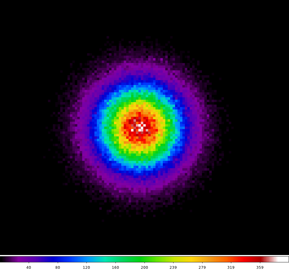
There are three dozens of a hot spot observations around the raw coordinates (rawx, rawy) = ( 14527, 7497) on HRC I. This hot spot is not a permanent one, but it often disappears for an extended period of time. It also changes its position slightly. We believe that this hot spot is created by a dust particle on MCP.
Since X-ray distributions created by the hot spot do not involve HRMA, we do not need to concern its point-spread function. Thus, the hot-spot observations provide a better data set when we need to adjust the parameters of the simulation model than real X-ray sources can.
) .
.
Before fitting a simulated model, we combined all hot spot observations into one data by centering the highest count pixel of each observation to the same center pixel. The resulted image is shown in Figure 8.
If you like to see individual observation image, please go to Hot Pixel Page.
Figure 9a shows the distributions of the hot spot data along X axis and Y axis. Fitted models are Voigt and Gaussian profiles. As before, the green line is Voigt model and the red is Gaussian model.
Table 2a lists the fitted parameters for Voigt profile; αD is the half width at half maximum for Doppler profile, αL is the half width at half maximum for Lorentz profile, ν0 is the central frequency, A is the area under profile, and a and b is the background as in a + b * x.
)
)
| X Axis | Y Axis | |
|---|---|---|
| αD | 1.166+/-0.162 | 1.169+/-0.044 |
| αL | 0.700+/-0.206 | 0.505+/-0.058 |
| ν0 | 0.089+/-0.030 | -0.050+/-0.009 |
| A | 3.951+/-0.250 | 3.574+/-0.068 |
| a | -0.012+/-0.010 | -0.007+/-0.003 |
| b | 0.0+/-0.0 | 0.0+/-0.0 |
We also fit Gauss-Hermite (GH) series model which is good for a skewed distribution (see the appendix). In Figure 9b, the blue line is GH model and the red line is Gaussian model. The GH model can represent X axis pretty well.
Table 2b lists the fitted parameters of Gauss-Hermite profile: γgh is the area covered (or integrated line strength), μgh is the mean abscissa, σgh is the dispersion, ξl is the skewness, and ξf is the kurtosis.
)
)
| X Axis | Y Axis | |
|---|---|---|
| γgh | 3.405+/-0.094 | 3.201+/-0.023 |
| μgh | 0.185+/-0.038 | -0.056+/-0.009 |
| σgh | 1.572+/-0.056 | 1.422+/-0.013 |
| ξl | 0.252+/-0.084 | -0.020+/-0.022 |
| ξf | 0.927+/-0.084 | 0.836+/-0.066 |
There are three variables in our simulations: ES ratio, pore overlapping, and the numbers of electrons generated by each hit, either by an X-ray or an electron. By changing these three variables, we can generate various shapes of distributions.
AR Lac fine position - center fraction relation is used to estimate ES ratio. We generated various data changing the ratio and found that ES ratio = 2.4 gives the best fit. This also gives reasonable fit on the hot spot data.
)
)
)
There is a suggestion that ES ratio is close to 1.5. We could fit ES =1.4 well on the data by changing the initial electron ejection speed from 4.2x10⁵ to 2.0x10⁵ m/s.
)
)
)
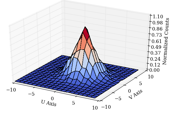
The following are example plots of a simulated data in two and three dimensional plots.
|
|
|---|
Voight profile is a combination of Lorentzian and Doppler broadening.
The convolution of both functions is
where
For more details, see Fitting Voigt Profiles
with
Integrated Line Strength:
Mean Abscissa:
Dispersion
Skewness
Kurtosis
For more details, see Fitting Gauss-Hermite series.