|
|
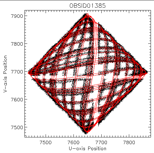
Figure 1: RAW positions of events from an 8-pixel radius
centered on AR Lac in ObsID 1385. The red over-plotted
curve shows the path of AR Lac based on an inversion of
the aspect solution.
|
Work by the LETG members of the calibration group has resulted in a method of correcting the dispersion relation via a lookup table. The CIAO tool hrc_process_events has been modified to use a lookup table for degapping rather than the fifth-order polynomial that has been in use since shortly after launch. While the correction values for the HRC-I lookup table can be populated by calculation using the current fifth-order polynomial, it would be beneficial if corrections for the "observed" deviations could be applied. Below I present a method for deriving improved degap corrections using the Chandra aspect solution to predict where a point-source should appear on the detector.
Just as a position on the detector can be mapped to the sky via the aspect solution, a position on the sky can be mapped back to a location on the detector by inverting the steps. The spacecraft dither will move an on-axis point source over a range of detector positions and the small PSF of that source will allow us to map the un-degapped, RAW event positions to a location on the detector. Figure 1 shows the path in RAW coordinates of events within a 8-pixel radius centered on AR Lac in ObsID 1385 as the spacecraft dithers. The horizontal and vertical breaks are the gaps produced by the loss of information intrinsic to the three-tap readout of the CGCD. The over-plotted red curve is the location of AR Lac as determined by inversion of the aspect solution as described below.
|
|
|
Figure 1: RAW positions of events from an 8-pixel radius
centered on AR Lac in ObsID 1385. The red over-plotted
curve shows the path of AR Lac based on an inversion of
the aspect solution.
|
For a given celestial source I invert the aspect solution through the following steps:
A bias can be introduced in the predicted detector locations by the first step. The event positions that we start with are affected by the residual errors in their positions. If the dither pattern is such that a significant number of events have large errors in a particular direction a bias in the derived mean position can be introduced that will propagate through to the predictions.
Starting with the events from the source and the aspect solution, the predicted source location on the detector can be calculated for every event. Then given a large number of events the mean RAWX (RAWY) coordinate can then be calculated for all events at a given U-axis (V-axis) position. With a large enough number of events at any location and a small enough region of source events selected the difference of the source location and the mean RAW coordinate is the degap amount that would be applied to the RAW coordinate. However, in working back from a predicted location on the detector we have to be careful around the gaps between tap centers. At the half-way point between taps events can produce RAW coordinates on either side of the gap and given a finite source event extraction size there will be events on the opposite side of the gap from the predicted source location. In addition, because of the incomplete ringing correction and possible mis-matching in the amplifiers, we should anticipate the possibility that there would be different degap corrections for different amplifier scale (AMP_SF) values. Accounting for these two issues results in differences between the mean RAW coordinate and predicted source location on the detector for events centered on a specific tap (CRSU or CRSV) and using a specific amplifier scale factor; figures 2 and 3 below show examples from the U- and V-axis, respectively.

|
| Figure 2: Mean of the differences between the modeled source location on the detector along the U-axis, derived from the aspect solution, and the reported RAWX value. Only events that were reported as centered on U-axis tap number 29 are included. Error bar sizes are calculated from the standard deviation of the differences divided by the square-root of the number of events with the predicted source position. Different colors are used to distinguish the values calculated from data with different amplifier scale factors (AMP_SF). Also plotted in the difference that results using the fifth-order polynomial degapping correction in the calibration database. |

|
|
Figure 3: Similar to figure 2 but for the V-axis with a V-axis
tap number of 30.
|
Events from sources from multiple observations or from multiple sources in a single observation can be combined to improve the statistics at a given location and to extend the coverage of position on the detector for which the degap value can be determined. Using multiple targets could help to minimize the potential bias discussed earlier by moving where on the detector the dither pattern samples. Including observations with non-standard SIM translation positions will also increase the areal coverage. As an initial trial in deriving degap correction for a lookup table I have used data from the ObsIDs given in the table below. The observations were selected to be nominally within 3 arcmin of on-axis and that were of sufficient duration and/or brightness to provide at least a few thousand counts in a 8-pixel radius extraction region around the source. ObsID 87 is an HRC-I/LETG observation where the zeroth-order events provide a large signal and which is one of the few observations with a non-standard SIM translation position. ObsID 6093 is another suitable observation with a non-standard SIM translation offset.
| ObsID | Object | SIM Z | Exposure | Number of Events | Y Offset | Z Offset |
|---|---|---|---|---|---|---|
| 87 | CYG X-2 | 122.980 | 29698.3 | 878527 | 0.0 | 0.0 |
| 461 | 3C 273 | 126.983 | 20097.0 | 206137 | 0.0 | 0.0 |
| 996 | AR Lac | 126.985 | 1318.3 | 3903 | 0.0 | 0.0 |
| 1000 | HZ43 | 126.985 | 3891.9 | 13130 | 0.0 | 0.0 |
| 1001 | HZ43 | 126.985 | 4955.0 | 17073 | 0.0 | 0.0 |
| 1286 | AR Lac | 126.983 | 873.1 | 2322 | 0.0 | 0.0 |
| 1321 | AR Lac | 126.985 | 984.5 | 2835 | 0.0 | 0.0 |
| 1382 | AR Lac | 126.985 | 789.1 | 2950 | 0.0 | 0.0 |
| 1385 | AR Lac | 126.985 | 19554.2 | 113820 | 0.0 | 0.0 |
| 1484 | AR Lac | 126.985 | 1287.8 | 6779 | 0.0 | 0.0 |
| 1485 | AR Lac | 126.985 | 1290.9 | 6651 | 2.0 | 0.0 |
| 1486 | AR Lac | 126.985 | 1287.9 | 5851 | 2.0 | -2.0 |
| 1487 | AR Lac | 126.985 | 1291.0 | 6743 | 0.0 | -2.0 |
| 1488 | AR Lac | 126.985 | 1287.8 | 5306 | -2.0 | -2.0 |
| 1489 | AR Lac | 126.985 | 1288.9 | 6031 | -2.0 | 0.0 |
| 1490 | AR Lac | 126.985 | 1287.8 | 4974 | -2.0 | 2.0 |
| 1491 | AR Lac | 126.985 | 1288.9 | 5846 | 0.0 | 2.0 |
| 1492 | AR Lac | 126.985 | 1289.8 | 4898 | 2.0 | 2.0 |
| 1514 | HZ43 | 126.985 | 2160.6 | 7501 | 0.0 | 0.0 |
| 1918 | GRS 1758-258 | 126.983 | 9949.8 | 38459 | 0.0 | 0.0 |
| 2345 | AR Lac | 126.985 | 1168.3 | 5246 | 2.0 | 0.0 |
| 2346 | AR Lac | 126.985 | 1191.6 | 4569 | 2.0 | -2.0 |
| 2347 | AR Lac | 126.985 | 1182.7 | 5449 | 0.0 | -2.0 |
| 2348 | AR Lac | 126.985 | 1194.1 | 4810 | -2.0 | -2.0 |
| 2349 | AR Lac | 126.985 | 1183.5 | 5682 | -2.0 | 0.0 |
| 2350 | AR Lac | 126.985 | 1196.6 | 5023 | -2.0 | 2.0 |
| 2351 | AR Lac | 126.985 | 1216.0 | 6011 | 0.0 | 2.0 |
| 2352 | AR Lac | 126.985 | 1198.5 | 4962 | 2.0 | 2.0 |
| 2604 | AR Lac | 126.985 | 1363.2 | 3014 | 2.0 | 2.0 |
| 2608 | AR Lac | 126.985 | 1189.5 | 5677 | 0.0 | 0.0 |
| 2609 | AR Lac | 126.985 | 1188.5 | 4564 | 2.0 | -2.0 |
| 2610 | AR Lac | 126.985 | 1193.8 | 5645 | -2.0 | 0.0 |
| 2611 | AR Lac | 126.985 | 1186.4 | 5314 | 0.0 | 2.0 |
| 2617 | AR Lac | 126.985 | 1186.4 | 5045 | 2.0 | 0.0 |
| 2618 | AR Lac | 126.985 | 1191.5 | 5197 | 0.0 | -2.0 |
| 2619 | AR Lac | 126.985 | 1188.5 | 3825 | -2.0 | 2.0 |
| 2624 | AR Lac | 126.985 | 1658.6 | 4395 | -2.0 | -2.0 |
| 3812 | CYG X-3 | 126.980 | 14694.0 | 133041 | 0.0 | 0.0 |
| 4288 | RXJ1856.5-3754 | 126.983 | 8442.2 | 13904 | 0.0 | 0.0 |
| 4290 | AR Lac | 126.985 | 1361.4 | 3006 | 2.0 | 2.0 |
| 4294 | AR Lac | 126.985 | 1176.9 | 5354 | 0.0 | 0.0 |
| 4295 | AR Lac | 126.985 | 1178.4 | 3928 | 2.0 | -2.0 |
| 4296 | AR Lac | 126.985 | 1175.7 | 4811 | -2.0 | 0.0 |
| 4297 | AR Lac | 126.985 | 1180.3 | 5171 | 0.0 | 2.0 |
| 4303 | AR Lac | 126.985 | 1179.7 | 5356 | 2.0 | 0.0 |
| 4304 | AR Lac | 126.985 | 1177.4 | 5191 | 0.0 | -2.0 |
| 4305 | AR Lac | 126.985 | 1167.3 | 4003 | -2.0 | 2.0 |
| 4310 | AR Lac | 126.985 | 1953.5 | 4200 | -2.0 | -2.0 |
| 5060 | AR Lac | 126.983 | 1137.4 | 5473 | 0.0 | 0.0 |
| 5061 | AR Lac | 126.983 | 1150.6 | 4688 | 2.0 | 0.0 |
| 5062 | AR Lac | 126.983 | 461.6 | 1654 | 0.0 | 2.0 |
| 5063 | AR Lac | 126.985 | 1060.6 | 3905 | -2.0 | 0.0 |
| 5064 | AR Lac | 126.985 | 1071.5 | 4000 | 0.0 | -2.0 |
| 5065 | AR Lac | 126.985 | 1082.8 | 3224 | 2.0 | -2.0 |
| 5066 | AR Lac | 126.985 | 1078.0 | 3194 | 2.0 | 2.0 |
| 5067 | AR Lac | 126.985 | 1083.0 | 2980 | -2.0 | 2.0 |
| 5068 | AR Lac | 126.985 | 1073.8 | 3395 | -2.0 | -2.0 |
| 6093 | GX13+1 | 76.978 | 8940.5 | 307285 | 0.0 | 0.0 |
| 6133 | AR Lac | 126.985 | 1076.7 | 5060 | 0.0 | 0.0 |
| 6134 | AR Lac | 126.985 | 1071.8 | 4796 | 2.0 | 0.0 |
| 6135 | AR Lac | 126.985 | 1569.3 | 4856 | 0.0 | 2.0 |
| 62507 | AR Lac | 126.985 | 1628.8 | 2031 | 0.0 | 0.0 |
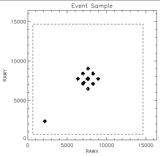
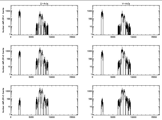
For each ObsID the tool hrc_process_events was re-run on the level 1 event list as necessary to apply all the latest corrections and obtain the current-best event positions. The center of the extraction region was determined by finding the centroid of the events within a 20-pixel-radius circle centered "by-eye" on the (near) on-axis source. The final events for analysis were selected using an 8-pixel-radius circle at the above determined centers and applying the standard status bits filter. Figure 4 shows the RAW positions of all the source events used while figure 5 shows histograms of the number of events at each modeled source position on the U- and V-axis and for the various AMP_SF values that were available for determining the mean RAW value. The events extracted here were also used to produce the difference data shown in figures 2 and 3. The extremely different SIM translation position of ObsID 6093 is clearly seen in the histograms as the peak to the left and illustrates how the entire raw coordinate range could be mapped using different SIM translation offsets with the dither pattern over-lapping between observations.
|
| Figure 4: RAW positions of selected source events used in determining values for the trial degap lookup table. The dashed line indicates the active area of the HRC-I. |
|
|
Figure 5: Histograms of the number of events as a function of
modeled position that were used in deriving the trial degap lookup table.
|
The links below are to plots similar to those in Figures 2 and 3 for
all of the coarse positions that have events from the combined
sources.
| CRSU: | 7 | 8 | 9 | 23 | 24 | 25 | 26 | 27 | 28 | 29 | 30 | 31 | 32 | 33 | 34 | 35 |
| CRSV: | 8 | 9 | 10 | 24 | 25 | 26 | 27 | 28 | 29 | 30 | 31 | 32 | 33 | 34 | 35 | 36 |
The degapping correction will be applied to the instrument RAW coordinate; however, the calculated differences (shown in figures 2 and 3) are of the mean RAW coordinate relative to the "corrected" location on the detector. The degapping correction at a given RAW coordinate can be obtained by interpolation or extrapolation of the calculated differences into a fixed grid of RAW coordinates using the mean RAW values for the modeled positions. The degapping corrections are placed into a lookup table with a RAW coordinate index; the tap number that supplies the differences used for a given range of RAW coordinates is the integer result of RAW/256 (i.e. CRSU = 29 is used for RAWX from 7424 to 7679). The places where this method of deriving a degap doesn't work, due to too few or no events, can be filled in using values calculated from the fifth-order polynomial degap coefficients in the calibration database.
For each coarse position and amplifier scale factor (AMP_SF) that had events from the combined, selected sources, I smoothed the calculated modeled-RAW differences by performing a running five-point weighted average of the differences. Only if the five consecutive modeled positions had data were they averaged and considered for further processing. A visual inspection of plots comparing the smoothed data to the input were used to decide if sufficient data existed in the range to continue. The modeled position - averaged difference pairs that were in the nominal coarse position range were then used to calculate a corresponding RAW position - difference pair and these pairs were interpolated to a fixed grid of RAW coordinates within the coarse position range using a least-squares quadratic fit to the four points surrounding the interpolate. I visually examined plots comparing the calculated deviations and interpolated degapping correction as a final quality check and rejected the segments that performed poorly (always due to too few events). The final candidate HRC-I degap lookup table is hrciD1999-07-22gaplookupN0002.fits I have used this file in CIAO 3.2 hrc_process_events to re-process the events for a few select observations; the resulting level 2 event lists can be obtained below:
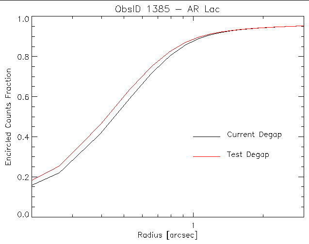
In each of these observations the central source is smaller than when using the current degap solution. As an example of the improvement, figure 6 shows a comparison of the encircled counts fraction profile of AR Lac from ObsID 1385 between event positions calculated using the current and candidate degaps.
|
|
Figure 6: Fractional encircled counts as a function of radius
for the on-axis source AR Lac (ObsID 1385). The black curve is the
resulting curve using the degap from the fifth-order polynomial, The
red curve is the result using the candidate degap derived by the
method described in this memo.
|
Last modified: Tue Aug 2 10:43:08 EDT 2005
Dr. Michael Juda
Harvard-Smithsonian Center for Astrophysics
60 Garden Street, Mail Stop 70
Cambridge, MA 02138, USA
Ph.: (617) 495-7062
Fax: (617) 495-7356
E-mail: mjuda@cfa.harvard.edu