|
This document describes the gain change correction algorithm which was derived for the CTI-corrected data in the FI chips and the uncorrected data in S3. This correction will be implemented in acis_process_events in a future release of CIAO. In the mean time, an equivalent standalone C program and calibration data is available from the Chandra software exchange page.
ACIS spectral response slowly evolves both because of changes in the CTI and evolution of the electronic gain in some of the CCDs. All relevant information can be found in C. Grant's presentation at 2002's Chandra calibration workshop: http://space.mit.edu/~cgrant/acis.html
Two different datasets are available for calibration of the time dependence of ACIS gain:
Our current approach is to derive the gain corrections from the ECS data and to verify their extrapolation to low energies by E0102-72 data. We use the ECS data integrated in a number of short observations spanning 3 months long periods starting in February 2000. This time resolution is adequate to sample the slow gain evolution (§ 3.3).
|
The released ACIS gain and RMF calibration was adjusted to the data taken in early 2000 (February-April), just after the ACIS focal plane temperature was lowered to −120 C. Using these calibration products, we derive the fractional change relative to these epoch by fitting the calibration data taken at later times.
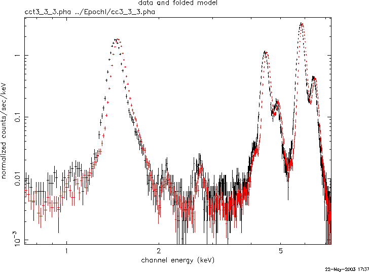
The ECS data are fitted with a model which has 6 Gaussian lines representing the main emission lines in the ECS spectrum. The ratio of the best-fit energies and the nominal energies gives the fractional gain change, ∆E/E, for the given epoch as a function of position.
The E0102-72 spectra are fitted with a physically motivated model consisting of an absorbed bremsstrahlung continuum and a number of emission lines whose energies and flux ratios are fixed based on the HETG observation. The model also includes two multiplicative factors to the line energies for O and Ne emission complexes. The best-fit values of these factors represent the gain change at E ≅ 0.6 keV (O) and ≅ 1.0 keV (Ne).
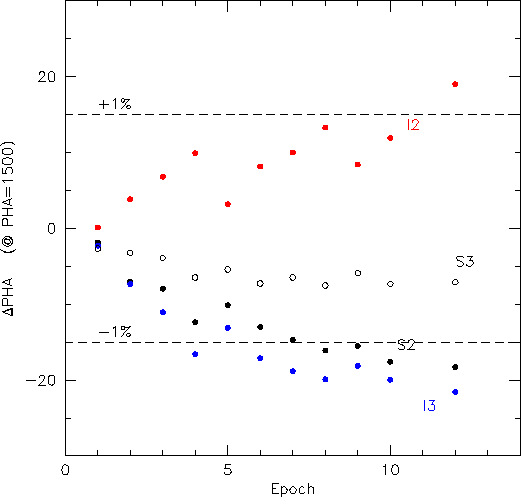
Figure 1 shows an example of CHIPY-dependence of the fractional gain change at E=1.49, 4.51, and 5.89 keV. To smooth out statistical uncertainties, we use the 4-th order polynomial fits shown by solid lines. Note that the fractional gain change increases at large distances from the readout and towards low energies.
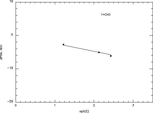
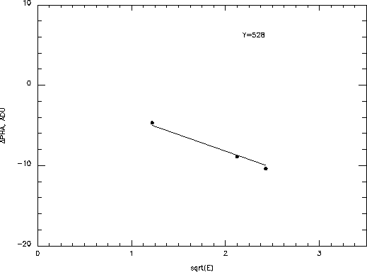
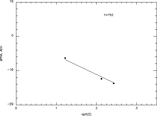
Using the released gain table, we can convert the fractional gain change (∆E/E) to the channel shift for each energy (∆PHA). Without changes in the internal electronics gain, ∆PHA represents the charge loss due to CTI. The phenomenological model of the CTI developed by the ACIS IPI team predicts that the energy dependence at each location is approximately ∆PHA = A E1/2. A similar energy dependence is indeed observed for the time-varying component of ACIS gain in most CCDs (Fig. 2).
|
 |
 |
At least one CCD (I2) shows strong variations in the internal electronics
gain on top of the increase in the CTI. Such changes can be represented by a
linear function of energy, ∆PHA = B E + C. Therefore, the
general function which describes the dependence of gain correction on energy
is
| (1) |
This is an over-determined model because we have to fit three coefficients to three data points. At present, we fix C=0 and B=0 in all CCDs except for I2 and S3. In I2, the internal gain evolution seems to be described by the BE term and so we fix C=0 and fit B in this CCD. In S3, the electronic gain is almost stable but there seem to be a secular zero-point drift by ∼ 2 ADU (http://space.mit.edu/~cgrant/acis.html). Therefore we fix B=0 and fit C in this CCD.
Equation (1) is fit to the data at 32 CHIPY steps for each node of the FI CCDs and for ∆CHIPX=32 steps in S3. Whenever B or C coefficients are needed, they are likely to be independent of CHIPY. Therefore, we average their best-fit values over the CHIPY steps and then refit the A coefficients with B or C held fixed.
The best-fit relation (1) is used to precompute the correction lookup tables, ∆PHA(PHA), for each location and epoch. A simple C program uses these tables to apply correction to the PHA values in either level1 or level2 event files.
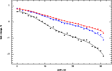
After Spring 2000, ACIS gain changes in most CCDs are slow (Fig. 3). Even at early times, the gain changes between the neighboring 3-month intervals are on the acceptably low (0.3% level).
|
External cal. source data do not show any detectable changes in the shape of the ACIS response except for the PHA shifts described above (e.g., Fig. 4 and 5).
|
 |
For a sanity check, we measured the locations of the bright Ka lines in the time-corrected ECS data. Since the corrections were derived from these data, the best-fit line energies should be very close to the nominal values. This is indeed achieved (see, e.g., the following table obtained for node 3 in I3 during Nov2002-Jan2003).
'% Diff' in the following table is defined as (E_measured-E_nominal)/E_nominal*100%

CCD: 3, NODE: 3,
        AlKa,1.487keV   TiKa,4.510keV   MnKa,5.898keV
yseg      % Diff          % Diff         % Diff
   0     -0.081          -0.120         -0.124
   1      0.054          -0.111          0.036
   2     -0.087          -0.089          0.010
   3      0.087          -0.111         -0.014
   4      0.101          -0.144         -0.073
   5     -0.128          -0.111         -0.044
   6     -0.101          -0.069         -0.049
   7     -0.262          -0.118         -0.090
   8     -0.081          -0.035         -0.063
   9     -0.027          -0.113         -0.066
  10      0.034          -0.100         -0.054
  11      0.007          -0.075         -0.061
  12     -0.027          -0.031         -0.109
  13     -0.161          -0.013         -0.088
  14     -0.155          -0.011         -0.088
  15      0.161          -0.129         -0.081
  16     -0.094          -0.086         -0.078
  17     -0.087          -0.084         -0.083
  18      0.182          -0.027         -0.078
  19      0.067           0.000         -0.073
  20      0.202          -0.109         -0.054
  21      0.027           0.000         -0.110
  22     -0.161          -0.206         -0.085
  23      0.047          -0.244         -0.122
  24     -0.020          -0.222         -0.129
  25     -0.148          -0.197         -0.137
  26      0.040          -0.047         -0.102
  27      0.256          -0.111         -0.110
  28      0.101           0.031         -0.070
  29      0.148          -0.111         -0.117
  30      0.175          -0.111         -0.163
  31      0.161          -0.222         -0.259
----------------------------------------------------------------
Mean      0.007          -0.097         -0.085
Standard  0.129           0.069          0.052
deviation
To verify the time-dependent gain correction at low energies we used the calibration observations of E0102-72. The summary of the results is given below. Essentially, the line energies for both O (E ≈ 0.6 keV) and Ne (E ≈ 0.9 keV) came out within 1% or better of their nominal values.
O_gain and Ne_gain in the following table are defined as the ratio of the
measured and nominal energies for the O and Ne complexes.

CCD     OBSID   Epoch   chipx    chipy          O_gain  Ne_gain
 I0     1542    VI      257:512  513:544        1.0075  0.9970
 I0     2840    VIII    257:512  513:544        1.0075  0.9970
 I1     444     I       1:256    97:128         1.0073  1.0040
 I1     445     I       1:256    481:512        1.0320  1.0240
 I1     1543    VI      257:512  481:512        1.0072  1.0060
 I1     2841    VIII    257:512  449:480        1.0073  1.0060
 I2     1544    VI      257:512  513:544        0.9990  0.9970
 I2     2842    VIII    257:512  513:544        1.0074  0.9970
 I3     1537    VI      1:256    481:512        0.9987  1.0025
 I3     2839    VIII    1:256    449:480        0.9988  0.9970
 I3     1536    VI      257:512  481:512        1.0073  0.9970
 I3     2838    VIII    257:512  449:480        1.0072  0.9970
 I3     420     I       513:768  97:128         1.0083  1.0100
 I3     140     I       513:768  289:320        1.0073  0.9970
 I3     136     I       513:768  449:480        1.0128  1.0140
 I3     1535    VI      513:768  481:512        1.0075  0.9970
 I3     2837    VIII    513:768  449:480        1.0074  0.9970
 I3     439     I       513:768  673:704        1.0085  1.0085
 I3     440     I       513:768  897:928        1.0048  0.9970
 I3     1533    VI      769:1024 97:128         1.0072  1.0060
 I3     2835    VIII    769:1024 97:128         1.0074  1.0060
 I3     1534    VI      769:1024 481:512        1.0075  0.9970
 I3     2836    VIII    769:1024 449:480        0.9988  0.9970
 S2     1539    VI      513:768  481:512        0.9988  0.9970
 S2     2847    VIII    513:768  481:512        0.9987  0.9970
The time-dependent gain correction will be implemented in the future release of acis_process_events. In the meantime, we provide a stand alone C program, corr_tgain.c. The only external library required by corr_tgain is CFITSIO which is widely distributed with FTOOLS.
Note also that corr_tgain should be applied to the CTI-corrected data in the I0-I3 and S2 chips (there is no reason to use uncorrected data in these chips!). The program will not modify the data for other FI CCDs and S1. Note that S0, S1, S4 and S5 are used primarily for grating observations so the time-depenedent gain change is less important.
Here is a typical data correction thread:
cp evt2.fits evt2-save.fits
Note that corr_tgain will change the PHA column in the events file and the original PHA values cannot be easily restored. Therefore, always save your data and run corr_tgain only once!
dmkeypar evt2.fits DATE-OBS ; pget dmkeypar value
2002-02-05T22:41:52
% ls corrgain*.fits
corrgain2000-01-29.fits  corrgain2001-02-01.fits  corrgain2002-02-01.fits
corrgain2000-05-01.fits  corrgain2001-05-01.fits  corrgain2002-05-01.fits
corrgain2000-08-01.fits  corrgain2001-08-01.fits  corrgain2002-11-01.fits
corrgain2000-11-01.fits  corrgain2001-11-01.fits
Select the latest file still appropriate for your data. For example, for the observation date above (February 5, 2002) the correct file is corrgain2002-02-01.fits. PHA correction is performed by the following command:
corr_tgain evt2.fits -tgain corrgain2002-02-01.fits
    acis_process_events\
    infile=evt2.fits\
    outfile=gov.fits\
    acaofffile=none stop=none\
    gainfile=/soft/ciao/CALDB/data/chandra/acis/bcf/gain/acisD2000-01-29gain_ctiN0001.fits\
    gradefile=none\
    apply_cti=no doevtgrade=no calculate_pi=yes check_vf_pha=no\
    clobber+

    mv gov.fits evt2.fits
Note that the corr_tgain calibration was derived for the CTI-corrected data in the FI chips. We expect that a similar correction applies to the non-corrected data as well. In this case the user should run corr_tgain as usual but use a different gain file on step 4.