Gallery: Smooth
Examples
- Smooth Image with Gaussian using FFT
- Smooth with rectangular box with sliding cell
- Smooth with Arbitrary Text Kernel
- Smooth with Image File
- Smoothing 3D Image
- Adaptive Smoothing with csmooth
- Adaptive Smoothing with dmimgadapt
- Adaptive smoothing with cone shaped kernel
- Circle With Minimum Number of Counts
- Gaussian Gradient Magnitude
- Directional Gradient Estimators
- Unsharp Mask
- Powerspectrum
- Deconvolution: arestore
1) Smooth Image with Gaussian using FFT
We start by simply convolving the input image with a circular, 2D Gaussian
aconvolve 635.img 635_gsm.img kernelspec='lib:gaus(2,5,1,3,3)' clobber=yes
The following commands can be used to visualize the output
ds9 635_gsm.img -scale log -zoom 0.6
The syntax for the aconvovle kernelspec parameter has four parts. The lib indicates that the smoothing kernel is to be constructed from one of the built in library functions. The gaus indicates the function to use: a Gaussian. The values in parentheses are the parameters for the Gaussian. It is a 2D Gaussian. The kernel should extend out to 5 sigma in each direction. The normalization is 1 (arbitrary here as the default is to recompute a normalization so that the volume under the kernel is 1). The final two parameter are the Gaussian sigma terms for the X and Y axes. This example does not include the optional fourth part of the kernelspec -- the location of the center of the smoothing kernel.
Based on this description, we see that this specifies that the data be smoothed by a 2D Gaussian with sigma=3.0 in both X and Y (ie, circularly symmetric) out to a radius of 5*sigma
2) Smooth with rectangular box with sliding cell
The aconvolve tool allows for smoothing kernels of arbitrary size. It also is not restricted to just smoothing images of the sky.
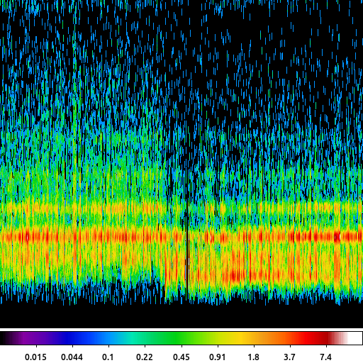
aconvolve cas_a.spectra.img cas_a.spectra.sm_img kernelspec="lib:box(2,1,1,10)" method=slide edge=const clob+
The following commands can be used to visualize the output
ds9 cas_a.spectra.sm_img -pan to 2200 230 physical -scale log -cmap sls
In this example, we take the image created in the Arbitrary Binning example where the X-axis is the region ID number and the Y-axis is the Energy. That image is smoothed with a 2D rectangular box that is only 1 pixel wide (X-axis) but 10 pixels long (Y-axis).
3) Smooth with Arbitrary Text Kernel
Sometimes it is useful to convolve with a simple, short array of numbers. For example a Laplace edge detector is given by a 3x3 matrix.
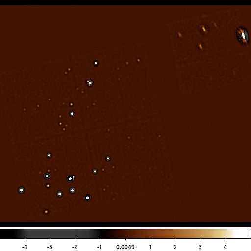
aconvolve 635_gaus.img 635_text.img kernelspec="txt:((-1,-1,-1),(-1,8,-1),(-1,-1,-1))" method=slide norm=none edge=const clob+
The following commands can be used to visualize the output
ds9 635_text.img -zoom 0.6 -scale limits -5 5 -cmap load $ASCDS_CONTRIB/data/heart.lut
In this example a version of the Laplace edge detection kernel is used by specifying a set of kernel values using the text, txt token. The values are given in nested parentheses, going from left-to-right, the values represent the bottom left pixel (first value), bottom middle pixel (2nd value), through the upper right pixel (9th value).
Unlike the previous examples we also have set the normalization parameter norm=none. This is because the sum of the pixels in the kernel is 0; so leaving the normalization at its default value would results in pixel values set to NaN.
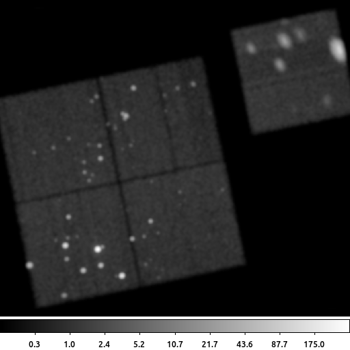
4) Smooth with Image File
The aconvolve tool can also convolve two images together using the kernelspec=file option.

The following commands can be used to visualize the output
ds9 15403.img 15403.psf 15403_file.img -tile mode column -frame 1 -zoom 2 -scale log -cmap bb -frame 2 -zoom 2 -scale log -cmap bb -frame 3 -zoom 2 \
    -scale log -cmap bb
In this example we use the arfcorr tool to create a quick, low fidelity, estimate of the Chandra PSF. The resulting image is saved in the file 15403.psf. This PSF is shown in the center frame.
We then use that image with aconvolve as the convolution kernel. The input image (shown on the left) is convolved with the PSF (center) to produce the output on the right.
Note: the input image and the PSF do not need to be the same size (MxN number of pixels); the PSF image can be smaller than the input image. However, the images must have the same resolution (pixel size) and tangent point.
5) Smoothing 3D Image
aconvolve supports multi-dimension images. This example shows a 3D image (cube) of a point source shown in chip coordinates. Since Chandra dithers during the observation, the point source moves across the detector versus time, which is the 3rd dimension.
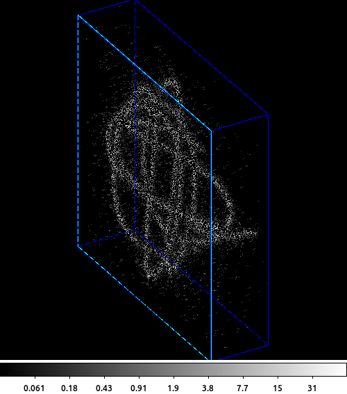
The following commands can be used to visualize the output
ds9 -3d smcube.fits -zoom 1.5 -scale log -view buttons yes -view info yes -3d az 60 -3d el 30 -frame delete 1 -sleep 5
The first step is to create the input data cube. Here an HRC event file is filtered on the chip coordinates and then binned into a cube. The X and Y axes are the chipx and chipy values binned by 2, and the third axis is time binned into 50 bins.
This cube is input into aconvolve. The convolution kernel used here acts like a delta function in the X and Y directions, and has an exponential decay along the Z (3rd/time) axis. The Lissajous pattern can be seen as the source dithers across the detector.
6) Adaptive Smoothing with csmooth
aconvolve does a linear smoothing. It smooths each pixel in the input with the same smoothing kernel. This works very well when all the interesting features in the input are approximately the same size and amplitude. However, when there are different size features (eg sources) with different amplitudes, a single linear convolution may be inadequate.
There are various adaptive smoothing techniques. They differ in performance; how smoothing scales are selected; figure of merit used to know when data are sufficiently smoothed (ie number of counts); etc.
CIAO includes the csmooth tool. This is an implementation of Harald Ebeling's asmooth algorithm. Using the default parameter settings, this algorithm smooths the data until the signal-to-noise in each pixel is between the input limits. It estimates the background from an annulus around each pixel; the size is based on the size of the kernel radius.
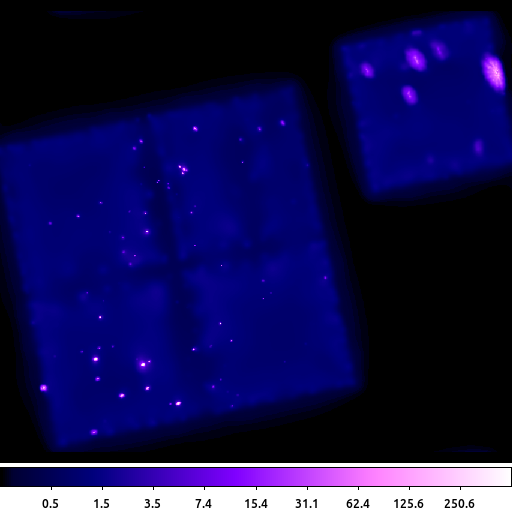
csmooth infile=635.img outfile=635_csm.img outsig=635_sig.img outscl=635_scl.img sigmin=3 sigmax=5 sclmax=45 clob+ mode=hl
The following commands can be used to visualize the output
ds9 635_csm.img -zoom 0.6 -scale log -scale limits 0 500 -cmap load $ASCDS_CONTRIB/data/purple4.lut
csmooth is fairly simple to run. It outputs the smoothed image as well as images that record the smoothing scale and the significance at each pixel location.
Users should be careful about how they use the output image. The flux in the image is not preserved (a local background has been subtracted.) There may also be some unphysical structure that emerges if there is significant structure in the background.
7) Adaptive Smoothing with dmimgadapt
CIAO also provides the dmimgadapt tools which does preserve flux. However, it does not estimate nor use a background in any way.
dmimgadapt may be a faster choice depending on the number of scales used. It also provides more choices in convolution kernels which can also greatly increase the speed.
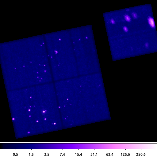
dmimgadapt 635.img out=635_adapt.img min=1 max=45 num=45 radscal=log fun=gaus counts=25 verb=3 clob+
The following commands can be used to visualize the output
ds9 635_adapt.img -zoom 0.6 -scale log -scale limits 0 500 -cmap load $ASCDS_CONTRIB/data/purple4.lut
This dmimgadapt output is a direct comparison to the csmooth example above. Both use a Gaussian convolution kernel to get approximately 5-sigma, ie 25 counts.
It's worth highlighting that the dmimgadapt tool knows about the filters which have been applied to the input file (aka the file's data-subspace). This is why the off-chip pixels appear white in this image -- they are actually NaN, whereas csmooth does not know about off-chip pixels, so the same area is filled with the value 0 (shown as black).
8) Adaptive smoothing with cone shaped kernel
While using a Gaussian is the most natural choice, it may not be the best option to start with. By definition, a Gaussian has infinite support (is non-zero everywhere). However, beyond some limit, the amplitude of the Gaussian is negligible. Most algorithms make an arbitrary cutoff, usually as a function of FWHM or sigma. Even so, the size of the Gaussian kernel may be quite large; leading to longer program runtimes.
dmimgadapt has several other smoothing kernel options which have finite support (identically 0 beyond some limit) and yet still retain the general shape of a Gaussian. Choosing one of these kernels can greatly reduce the program's runtime, which can be especially useful when doing exploratory analysis trying to determine the range of other input parameters to use.
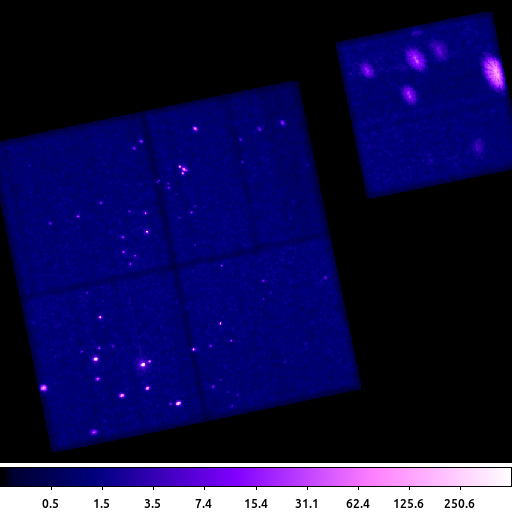
dmimgadapt 635.img out=635_adapt_cone.img min=1 max=45 num=100 radscal=log fun=cone counts=16 verb=3 clob+
The following commands can be used to visualize the output
ds9 635_adapt_cone.img -zoom 0.6 -scale log -scale limits 0 500 -cmap load $ASCDS_CONTRIB/data/purple4.lut
This example shows dmimgadapt using the circular cone shaped kernel. This example uses more smoothing kernels than the previous example; and yet because the cone is easier to compute and has a finite base, the dmimgadapt program runs much faster.
Visually this image is nearly identical to the previous example. Since selecting the set of smoothing kernel scales is often an iterative task, we can use the cone kernel to quickly optimize those parameters first and then run again using gaus to produce the final product.
9) Circle With Minimum Number of Counts
The primary output from dmimgadapt is usually the smoothed image. However, it also provides a map with the size of the smoothing kernel radius as well as the SNR and normalization.
The radius map can be very useful for various types of analysis. Consider the case of doing spectral fitting where we require a minimum number of counts to get reliable fit results. We may need to know the size of a circle centered at each pixel location that encloses, for example, at least 100 counts. This is easy to get using dmimgadapt.
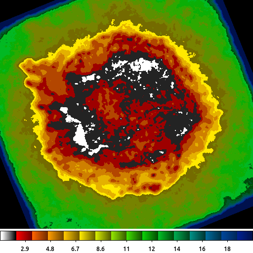
dmimgadapt 214.img out=214_adapt.img min=1 max=20 num=20 radscal=linear fun=tophat counts=100 verb=3 radfile=min_100cts.map clob+
The following commands can be used to visualize the output
ds9 min_100cts.map -zoom 1 -linear -cmap load $ASCDS_CONTRIB/data/16_ramps.lut -view colorbar yes
The image shown is the min_100cts.map file. Note that units of the radii are in logical pixels, so if an image is binned > 1, which is the case here, you want to be sure to take that into account when using this file.
See also the Find regions with minimum number of counts thread.
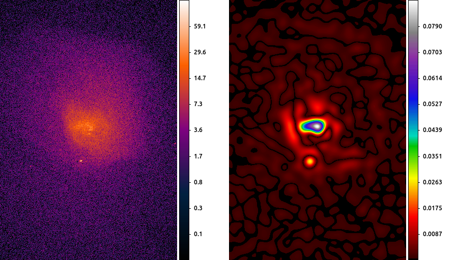
10) Gaussian Gradient Magnitude
The Gaussian Gradient Magnitude algorithm is becoming increasingly popular in astronomy image processing. The derivative of a Gaussian is an effective edge detector which suppresses high-spatial frequencies, most often associated with the background.
We can make use of the convolution identity:
\[ I \ast \nabla h = \nabla (I \ast h) \]where I is the input image and h is a Gaussian. This means that rather than trying to compute the partial derivatives of a Gaussian; we only need to convolve the image with a Gaussian, and then compute the image gradient.
The gradient of an image can be estimated by convolving it with a specially constructed convolution kernel; for example the Laplace kernel = ((0,1,0),(1,-4,1),(0,1,0))
As shown here, the GGM is then easy to compute by running aconvolve twice. dmimgcalc is then used to compute the magnitude of the gradient estimator; which here is just the absolute value of the gradient (the factor of sqrt(2.0) is included for completeness.)
The following commands can be used to visualize the output
ds9 abell496_broad_thresh.img abell496_ggm.img -frame 1 -scale log -pan to 4065 3890 physical -cmap load $ASCDS_CONTRIB/data/gem-256.lut -frame 2 \
    -scale linear -pan to 4065 3890 physical -cmap load $ASCDS_CONTRIB/data/iman.lut -view colorbar on -colorbar vertical
In this example we start by smoothing the image with a 10 pixel Gaussian, and then estimating the gradient using the Laplace convolution kernel. The result here shows a cavity North of the center of the cluster which can then be further analyzed.
The choice of the smoothing scale affects the size of detectable features. To look for large scale features, a large smoothing scale is required. The scale should always be larger than the local PSF size. Since the Chandra PSF varies, some researchers have found innovative ways to combine GGM from several scales into a single product.
11) Directional Gradient Estimators
In the previous example we used the Laplacian gradient estimator. The nice thing about this estimator is that it can be computed with a single convolution. However, it only contains information about the magnitude of the gradient, not the direction. To get directional information about the gradient, we have to use other gradient estimators.
One of the most common gradient estimators is the Sobel kernel. There is a separate convolution kernel designed to estimate the gradient in the X-direction and in the Y-direction. These then just need to be combined together to get the magnitude and the angle of the gradient.

aconvolve abell496_gaus10.img abell496_dx.img "txt:((1,2,1),(0,0,0),(-1,-2,-1))" meth=fft clob+ norm=none
aconvolve abell496_gaus10.img abell496_dy.img "txt:((-1,0,1),(-2,0,2),(-1,0,1))" meth=fft clob+ norm=none
dmimgcalc abell496_dx.img,abell496_dy.img none abell_sobel.mag op="imgout=sqrt((img1*img1)+(img2*img2))" mode=h clob+
dmimgcalc abell496_dx.img,abell496_dy.img none abell_sobel.ang op="imgout=atan(img2/img1)" mode=h clob+
The following commands can be used to visualize the output
ds9 abell_sobel.mag abell_sobel.ang -frame 1 -zoom 0.5 -scale log -cmap h5_bone -frame 2 -zoom 0.5
In this example we used aconvolve to compute the directional gradient in the X-direction and separately in the Y-direction. Then dmimgcalc is used to compute the magnitude (left) and angle (right) of the gradient. The data are the same shown in the Gaussian Gradient Magnitude example , but zoomed out by 50%. The edge of the cluster emission is easy to identify in the gradient magnitude image (left). The gradient direction image (right) is harder to interpret since the angle wraps at 180 degrees, creating an artificial discontinuity.
Some other common gradient estimators include:
| Name | X | Y |
|---|---|---|
| Laplace | ((0,1,0),(1,-4,1),(0,1,0)) | ((0,1,0),(1,-4,1),(0,1,0)) |
| Sobel | ((1,2,1),(0,0,0),(-1,-2,-1)) | ((-1,0,1),(-2,0,2),(-1,0,1)) |
| Roberts | ((1,0),(0,-1)) | ((0,1),(-1,0)) |
| Prewitt | ((1,1,1),(0,0,0),(-1,-1,-1)) | ((-1,-1,-1),(0,0,0),(1,1,1)) |
| Robinson | ((1,1,1),(1,-2,1),(-1,-1,-1)) | ((-1,1,1),(-1,-2,1),(-1,1,1)) |
| Kirsch | ((3,3,3),(3,0,3),(-5,-5,-5)) | ((-5,3,3),(-5,0,3),(-5,3,3)) |
12) Unsharp Mask
Unsharp masks have been used by photographers for decades to improve the contrast of photographs. This technique involves slightly blurring the original image, inverting it, and adding a scaled version of the inverted, blurred image back to the original image. The result is that edges become more pronounced and visually appealing.
Mathematically this looks like:
\[ U = I - I\ast h \]Where I is the original image, h is the smoothing function (usually a Gaussian), and U is the unsharp mask. Since a Gaussian is a low pass filter (it tends to preserve large spatial features), by subtracting the smoothed image from itself we are then accentuating small scale features such as edges or boundaries between objects (ie high spatial frequencies). Unfortunately, this may also adversely accentuate the noise. Therefore, rather than subtract the smoothed image from the original, often it is subtracted from a the image smoothed with a different size Gaussian.
\[ \hat{U} = I \ast g - I\ast h \]If we require that the spatial scale of g by smaller than h, then what we end up with is a spatial band-pass filter that is sensitive to spatial features larger than g but smaller than h. This has the advantage of accentuating spatial features at some spatial scales while suppressing the noise.

The following commands can be used to visualize the output
ds9 abell2390.img abell2390_unsharpmask.img -frame 1 -scale log -cmap load $ASCDS_CONTRIB/data/brain.lut -frame 2 -scale log -cmap load \
    $ASCDS_CONTRIB/data/heart.lut -view colorbar on
The choice of how large to make g compared to h is discussed in the literature. One common convention is to use a factor 10, so if g is a Gaussian with a 3 pixel sigma, then h should be a Gaussian with a 30 pixel sigma. Other researchers have used various other values (5 and 20).
Finally, we can rearrange the terms above to get
\[ \hat{U} = I \ast (g - h) \]We can then identify the term (g-h) as the difference of Gaussians (DoG). There has been research in this specific topic as the DoG can be used to approximate the Haar (aka Mexican Hat) wavelet. Given this relationship, some users will select scales at 2n radii.
13) Powerspectrum
In the previous example we talked about the unsharp mask as a band-pass filter, we can see that by looking at the power spectrum (the magnitude of the Fourier transform) of the output.
apowerspectrum abell2390_unsharpmask.img infileimag=none outfile=powerspectrum.img clob+ center+
The following commands can be used to visualize the output
ds9 powerspectrum.img -scale asinh -cmap b -zoom 2
In this example the power spectrum has been centered such that the middle of the image represents the lowest spatial frequencies (ie the "flat" background) and the highest frequencies are at the edge of the image.
What we see here is an annulus with little power at high frequencies due to the 3 pixel Gaussian filter and littler power at low frequencies due to the subtraction of the 30 pixel Gaussian smoothed image. This annulus is the frequency band-pass represented in the unsharp mask filtered image.
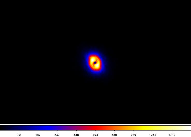
14) Deconvolution: arestore
Blind deconvolution techniques also rely on convolution. In the Richardson-Lucy deconvolution technique, available in the arestore tool, the image is repeatedly convovled with the PSF and then subtracted from itself. The effect is similar to the unsharp mask being applied repeatedly.

simulate_psf hrcf10578N003_evt2.fits ar_lac ra=332.1699988 dec=45.7422877 monoenergy=1.0 flux=1.0e-3 numiter=10 minsize=256 rand=5678 mode=h
get_sky_limits ar_lac.psf
dmcopy "hrcf10578N003_evt2.fits[bin X=16150.5:16406.5:#256,Y=16288.5:16544.5:#256]" ar_lac.img clob+
arestore ar_lac.img ar_lac.psf ar_lac.deconvolve numiter=250 clob+
The following commands can be used to visualize the output
ds9 ar_lac.img ar_lac.psf ar_lac.deconvolve -frame 1 -scale log -zoom 4 -cmap load $ASCDS_CONTRIB/data/yellow1.lut -frame 2 -scale log -zoom 4 -cmap \
    load $ASCDS_CONTRIB/data/green7.lut -frame 3 -scale log -zoom 4 -cmap load $ASCDS_CONTRIB/data/brown.lut -tile mode column
In this example we used the simulate_psf script to run MARX to simulate the PSF at the location of ArLac (center image). We then used the get_sky_limits script to get the limits used to bin the PSF image and use that with dmcopy to make the image of the data (left image). Finally, we used arestore to perform the Lucy-Richardson deconvolution technique with 250 iterations for the deconvolved image (right image).
There appears to be excess flux North of the source. While it may be tempting to think that this is some extended source emission, there are several factors to consider such as the energy used in the PSF simulation and the existence of a known PSF artifact, which can be located using the following command
make_psf_asymmetry_region ar_lac.img anomaly.reg x=16277.5 y=16416.1 format=ds9 clob+
and loading the region onto the deconvolved image.